Sampled Data Aliasing

In the Sampled Data example, a 3 kHz sine wave signal was sampled at 48 kHz. That sample rate was 16 times the signal frequency, and we captured a fair representation of the sine wave signal.

But suppose we cut the sample rate to 6 kHz, only twice the signal frequency; in that case, the sampled data (large open squares) would fall on the equivalent of every 8th sample of the original data:

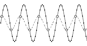
Now we are only getting 2 samples per cycle of the input wave. Given only the new sampled data, the "best guess" at the true input wave would be the dotted curve connecting the open squares. Clearly, this does not give a proper representation of the true signal amplitude, although in this case it does give the proper frequency. In fact, if the relative phase between the signal and the sampling were changed (by starting on another sample of the original, or sampling at any other point on the wave), we could get any amplitude from the proper value down to zero.

This half-the-sample-rate signal is at the so-called Nyquist frequency. Since at this frequency we can't rely on the sampled data to reconstruct the input signal, this is often referred to as the Nyquist limit for a sampled data system.

But suppose the sample rate in our example is reduced from 48 kHz to 2666.7 Hz, a factor of 18. The new samples (larger open squares) coincide with every 18th sample of the original data:

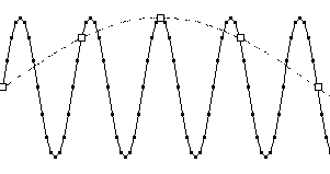
Now there is less than one sample per cycle of the input wave. Without knowing the actual frequency of the input, the best-guess fit to this new data would be the dotted curve connecting the open squares. Since this apparent or alias wave takes 4 samples to go through a half cycle, or 8 for a full cycle, we would assume that the input frequency is 2666.7 / 8 = 333.3 Hz. The frequency measurement would thus be in error by a factor of nine! A DFT would give this same erroneous result.

Such alias signals arise whenever a component of the input signal is more than the Nyquist frequency. This is sometimes known as the "folding frequency", because the effect is as though you had folded the true spectrum about that point, causing high frequency components to appear down at the low end of the spectrum. This is actually a pretty good analogy, since it allows you to figure out where those aliased components will appear.

For example, if the Nyquist frequency is 24 kHz (sample rate of 48 kHz), then input components under 24 kHz will appear at their proper locations on a spectrum display. But a 25 kHz input will be folded about the 24 kHz point, so it will appear as an alias at 23 kHz.

If you scroll the input frequency up from zero, a real-time spectrum will show a single peak that moves up until it "hits" the Nyquist frequency and "bounces off". As you continue to increase the input frequency, this peak will now move down toward the low end. The peak will hit zero frequency (DC) when the input is just at the sample frequency, and if you keep scrolling upward the peak will bounce back and continue upward.

Given a known input and sample rate, you can figure out where the alias will appear on the spectrum. Divide the input frequency by the Nyquist, and look at the integer portion of the quotient. If it is 0, the input will be shown properly, with no alias. If the integer is odd, you'll get an alias that is coming down from the Nyquist by the fractional part of the quotient (in other words, at the Nyquist frequency times one minus that fraction.) If the integer is even, the alias will be coming up from zero by that fraction of the Nyquist.

In the previous example, 25 kHz / 24 kHz = 1.0417, since the integer is odd we know the alias will be coming down from the Nyquist. Its exact location will thus be (1 - 0.0417) * 24 kHz = 23 kHz.

An input at 49 kHz would give 49 / 24 = 2.0417, and since the integer is even the alias would appear at 0.0417 of the Nyquist or 1 kHz.

Note that you can't work this rule backward to find an unknown input frequency given an observed peak: You can't even tell a priori that a peak is an alias, let alone how many times it has been folded over or whether it's on an odd or even fold. That's part of the danger of aliases.

When the input is exactly at the Nyquist frequency, or any multiple of it, the input level is indeterminate. Consider that at half the sample rate there will only be two samples per cycle, and (except for certain synchronous sampling systems) the phase will be unknown. So those two samples could come at the positive and negative peaks, or two zero crossings, or anywhere in between... you just don't know. (That's why spectrum analyzers don't usually show a line corresponding to the Nyquist frequency; it wouldn't have much meaning in most cases.)

It should be clear from the above that to prevent aliased components from giving erroneous results, the input signals, including harmonics of complex waveforms must be limited to less than the Nyquist frequency. This is not just a problem related to viewing spectra... these aliased signals would be clearly audible if we simply played back such an undersampled data stream. And since aliases of harmonic frequencies would no longer be related to the fundamental, the inharmonic sound would be particularly unpleasant, like serious intermodulation distortion.

Since aliasing is such a serious problem, and since we often have input signals with lots of upper harmonics, sound cards always incorporate anti-aliasing filters to drastically reduce any components above the Nyquist limit. Note that the aliasing effect arises at the time of sampling; once the data is sampled and an alias is produced, there is no feasible way to filter out the aliases... they are indistinguishable from real input signals that just happened to fall on those frequencies.

So the anti-aliasing filter must be a real hardware filter ahead of the ADC; it can't be implemented by purely digital means after sampling.

Anti-alias filters must be carefully chosen in order to avoid other problems with your data. A filter which sharply reduces frequencies above its "cutoff" will usually also cause phase shifts which can alter the appearance of the waveform, even if they don't affect the spectrum. Further, transient inputs may provoke waveform overshoot and ringing behavior, due to Gibbs phenomenon.

Naturally, the types of filters that are least prone to these problems also don't have very sharp cutoffs unless they are made very complex. Here complexity is measured by filter "order", which is the number of tuned stages required. Since each tuned stage requires precision components, and since the required precision (and stability over time) increases with the filter order, sound cards that used such filters would be quite expensive.

Fortunately, there is a way to use a simple, inexpensive filter together with more sophisticated digital processing to get results superior to even the most complex hardware filters. Modern sound cards typically use a delta-sigma ADC (sometimes called sigma-delta) that runs at a very high input sample rate, but with low initial bit-resolution. This high-speed, low-bits digital stream is then filtered and resampled by purely digital means to yield the final output, with high resolution at the stated sample rate (like 48000 Hz).

Because the initial sample rate is so high, in the hundreds of kilohertz to megahertz range, the Nyquist frequency will be far removed from the region of the input signals. A simple analog filter is all this type of ADC may need at its input, since there are usually no input signal components near these extreme frequencies.

The real work of removing problem frequencies (those that would have caused aliasing in a conventional ADC) comes during digital resampling to the lower rate. By then the signal is already in digital form, so a very sharp digital filter can be employed right in the ADC chip. In fact, it may be an inherent part of the resampling process, at "no extra charge".

We have so far been discussing the aliases that arise when we sample analog signals to create a digital version, but the same situation happens in reverse, when a Digital-to-Analog Converter (DAC) tries to generate a wave with harmonics higher than the Nyquist rate. Thus, sound cards also incorporate output filters (often called anti-imaging or reconstruction filters) as well as input filters.

See also Aliasing Demonstration, Spectrum (Fourier Transform) Theory