Software for Windows
Science with your Sound Card!
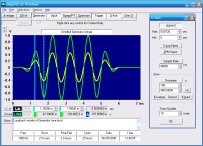
Features:
Oscilloscope
Spectrum Analyzer
8-Channel
Signal Generator
(Absolutely FREE!)
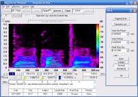
Spectrogram
Pitch Tracker
Pitch-to-MIDI
DaqMusiq Generator
(Free Music... Forever!)
Engine Simulator
LCR Meter
Remote Operation
DC Measurements
True RMS Voltmeter
Sound Level Meter
Frequency Counter
Period
Event
Spectral Event
Temperature
Pressure
MHz Frequencies
Data Logger
Waveform Averager
Histogram
Post-Stimulus Time
Histogram (PSTH)
THD Meter
IMD Meter
Precision Phase Meter
Pulse Meter
Macro System
Multi-Trace Arrays
Trigger Controls
Auto-Calibration
Spectral Peak Track
Spectrum Limit Testing
Direct-to-Disk Recording
Accessibility
Data Logger
Waveform Averager
Histogram
Post-Stimulus Time
Histogram (PSTH)
THD Meter
IMD Meter
Precision Phase Meter
Pulse Meter
Macro System
Multi-Trace Arrays
Trigger Controls
Auto-Calibration
Spectral Peak Track
Spectrum Limit Testing
Direct-to-Disk Recording
Accessibility
Applications:
Frequency response
Distortion measurement
Speech and music
Microphone calibration
Loudspeaker test
Auditory phenomena
Musical instrument tuning
Animal sound
Evoked potentials
Rotating machinery
Automotive
Product test
Contact us about
your application!
EQ_Curve - Equation-to-Curve Mini-App
- Introduction
- Transfer Function Basics
- A Simple Low-Pass Filter
- A Simple High-Pass Filter
- Poles and Zeros
- Frequency Response and Bode Plots
- Setting EQ_Curve Parameters
- Using EQ_Curve
- EQ_Curve Macro Listing
- _EQ_Core Macro Listing
Introduction:
The EQ_Curve macro mini-app is included with Daqarta. It computes and displays a transfer function curve from its parameters, and allows you to save it as a Weighting Curve file for use with the Spectrum Curves option.
Unlike most other included mini-apps, EQ_Curve requires you to modify the first section of the macro itself in order to specify the desired curve. Examples of several such sections are provided for standard weighting curves (A-Weight through D-Weight, plus RIAA and IEC-RIAA and their inverses), as well as several conventional filters.
For other curves, you need to know the parameters of the desired transfer function. EQ_Curve allows you to enter these in a variety of formats, and takes care of the conversions for you. This allows you to use parameters in the same format you find them in from various technical sources, without needing error-prone manual conversion.
Transfer Function Basics:
(Skip the next few sections if you are already familiar with transfer functions and corner frequencies.)
For our purposes here, a transfer function is a mathematical expression that characterizes the frequency response of a system. It represents the ratio of the output voltage of a system divided by its input, as a function of frequency. Consider a simple voltage divider:
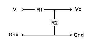
Its transfer function is simply:
K = Vo / Vi = R2 / (R1 + R2)
Since resistors are not frequency-dependent, K is a constant, not a function of frequency.
A Simple Low-Pass Filter:
Compare the above to a simple low-pass filter made from a resistor R and capacitor C:
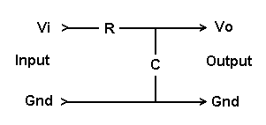
This has the form of a voltage divider, such that the ratio of output voltage to input voltage K is given by:
K = Zc / (R + Zc).
Zc is the impedance or reactance of the capacitor, effectively its "AC resistance". (We assume that the divider is driving an infinite impedance, so we don't need to consider that here.)
Zc is inversely proportional to frequency, so at high frequencies it acts like a low resistance and greatly reduces the output of the voltage divider. At low frequencies Zc acts like a high resistance; the input signal passes to the output with little loss from the divider... hence the designation "low-pass".
At some intermediate frequency, Zc will have the same value as the resistance R. In a normal resistor-only voltage divider with equal-value resistors, the output voltage would be exactly half of the input voltage, or -6 dB. But that doesn't happen here, because reactance also has a phase associated with it. (For a capacitor, the phase of the current through it is always 90 degrees from the AC voltage across it.)
To account for phase, AC circuits use complex numbers to represent sine wave signals and impedances. A complex number may have a real part and an imaginary part, written in the form A + jB. The imaginary number j is the square root of -1. (Mathematicians typically use i for this, but engineers use j to avoid confusion because i is used for current.)
The impedance of a resistor is purely real, with a value of R ohms and no imaginary part. The impedance of a capacitor is purely imaginary, with a value of Zc = 1 / jwC. Here the 'w' represents small omega, which is the frequency in radians per second. Since there are 2 * pi radians in one revolution or cycle, w = 2*pi*F where F is the frequency in hertz (cycles per second).
If we plug this complex Zc into the voltage divider formula K = Zc / (R + Zc), we get:
H(jw) = 1/jwC / (R + 1/jwC)
Note that we replace K with H(jw). H is a standard notation for transfer function, and H(jw) denotes that it is a function of complex frequency jw.
Multiplying numerator and denominator by jwC we get:
H(jw) = 1 / (R * jwC + 1)
As it turns out, the product of a resistance and a capacitance has units of seconds. If we define w0 = 1 / (R * C) we get:
H(jw) = 1 / (jw/w0 + 1)
Multiplying numerator and denominator by w0 gives:
H(jw) = w0 / (jw + w0)
We are interested in the frequency amplitude response of this low-pass filter (as opposed to phase response, so we need to find the magnitude of the above complex expression. The magnitude of a complex number like jA + B is sqrt(A^2 + B^2), so the magnitude response |H(jw)| is:
|H(jw)| = w0 / sqrt(w^2 + w0^2)
Note that at frequencies where w is much smaller than w0, the above approaches unity. At frequencies where w is much larger than w0, the above approaches w0 / w... the output voltage is halved when the frequency is doubled. In dB terms, it falls by 6 dB for each doubling, denoted as 6 dB/octave. (An octave is a doubling of frequency.) This describes a simple low-pass filter.
Here is an example EQ_Curve plot for such a filter where w0 is equivalent to 3000 Hz. You can see the 6 dB change in the octave between 10 kHz and 20 kHz, but not at lower frequencies... there w is still too close to w0, not big enough to be "much larger".
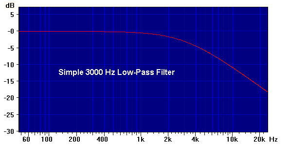
At 3000 Hz, the frequency where w = w0, the magnitude is:
    |H(jw)| = w0 / sqrt(w0^2 + w0^2)

    |H(jw)| = w0 / sqrt(2 * w0^2)

    |H(jw)| = w0 / (sqrt(2) * w0)

    |H(jw)| = 1 / sqrt(2)

    |H(jw)| = 0.707107...
Converting this voltage ratio to dB we get:
20 * log10(0.707107) = -3.0103 dB
This is shown in the above image, where the curve is down to about -3 dB at the 3 kHz point.
It turns out that w0 is the frequency where the magnitude of the reactance of C equals the resistance of R, which as we previously noted is not where the output voltage is halved as in a simple resistive divider.
w0 is termed the "corner frequency" or "break point" of the transfer function. When plotted as dB (log Y) on a log frequency (log X) axis, it is the intersection of the horizontal asmyptote of the 0 dB line of the flat low-frequency reponse portion, with the -6 dB/octave asymptote of the high-frequency portion.
A Simple High-Pass Filter:
A simple high-pass filter can be formed by exchanging the positions of the resistor and capacitor:

This changes the underlying voltage divider from:
K = Zc / (R + Zc)
to:
K = R / (R + Zc)
Since Zc is inversely proportional to frequency, at low frequencies where it acts like a high resistance the output of the divider is greatly reduced. At high frequencies where Zc is negligible compared to R the above approaches R / R and the input passes to the output with little loss... a "high-pass" filter.
Substituting 1/jwC for Zc gives:
H(jw) = R / (R + 1/jwC)
Multiplying numerator and denominator by jwC we get:
H(jw) = R * jwC / (R * jwC + 1)
Using w0 = 1 / (R * C) produces:
H(jw) = jw/w0 / (jw/w0 + 1)
Multiplying numerator and denominator by w0 gives:
H(jw) = jw / (jw + w0)
The magnitude of this is:
|H(jw)| = w / sqrt(w^2 + w0^2)
At high frequencies where w is much larger than w0, the above approaches w / w = 1 to give the "high-pass" part of the response. At low frequencies where w is much smaller than w0, the above approaches w / w0 and the response is directly proportional to frequency; the response rises up toward the flat portion at +6 dB/octave.
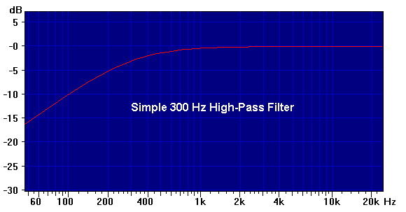
Here is an example EQ_Curve plot for such a filter where corner frequency w0 (the -3 dB frequency) is equivalent to 300 Hz. You can see the 6 dB change in the octave between 50 and 100 Hz, but not at higher frequencies... there w is still too close to w0, not small enough to be "much smaller".
Note that the high-pass equation is identical to the low-pass version, except the numerator is now frequency w instead of constant w0. One way to interpret this is that the numerator w contributes a +6 dB/octave slope at all frequencies, while the denominator adds a -6 dB/octave slope above w = w0 that flattens it to 0 dB/octave to form the high-pass region.
Poles and Zeros:
The above simple low-pass and high-pass filters demonstrate some general features that can be used (with a few others) to analyze all kinds of transfer functions. But first we will take a detour into standardizing: Engineers typically use a shorthand Laplace transform notation for transfer functions, using s to represent jw. For the simple high-pass:
    H(jw) = jw / (jw + w0)

    H(s) = s / (s + w0)

    |H(s)| = s / sqrt(s^2 + w0^2)
Here we will consider only the general H(s) non-magnitude form, from which we can obtain either the magnitude or phase response as needed. Complicated transfer functions can be factored into the general format of a product of numerator terms divided by a product of denominator terms. Here is an example:
            s^2 * (s + w0) * (s + w1)
    H(s) = ---------------------------
             (s + w2) * (s + w3)^4
The numerator terms are called zeros; you can remember this by noting that if a numerator term evaluates to zero at any frequency (such as the initial s^2 at zero frequency = DC), the whole function will go to zero.
The denominator terms are called poles; if any of these evaluates to zero, the overall function entails a division by zero which causes the output to go to infinity... a vertical "pole" in the response plot.
A term that is repeated exactly may be replaced by a single term raised to a power, as with the s^2 term (two zeros at DC) in the numerator and the (s + w3)^4 term in the denominator (four poles at w3 corner frequency). The exponent of s is the order of that term.
We've already seen the single s zero-at-DC form in the simple high-pass filter, and the (s + w0) form with a corner frequency as a pole in both the high-pass and low-pass filters. Either form can be in the numerator as a zero, or in the denominator as a pole.
A Simple Band-Pass Filter:
Consider a simple band-pass filter which is a combination of a simple high-pass section with w0 equivalent to 300 Hz, and a simple low-pass with w1 equivalent to 3000 Hz.
                    s
    H(s) = --------------------
           (s + w0) * (s + w1)
Note, however, that this assumes that the high-pass and low-pass stages are independent; each must be driven by a low impedance, and must drive a high impedance. That implies that there must be a buffer amplifier between these stages. Otherwise, the simple voltage divider model used for each stage will not be correct, since the second stage will load down the first.
This added amplifier is normally not an issue since most filters have amplification stages in them anyway. These are called active filters, as opposed to those that use only passive components like resistors, capacitors, and inductors.
(In this simple example, you could get around the need for the amplifier by using a small resistor in the high-pass first stage, and a large resistor in the low-pass second stage... typically 10 times larger to prevent loading effects. Then you'd have to select the proper capacitor values according to the original high-pass and low-pass formulas.)
Here's the response plotted by EQ_Curve:
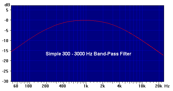
You may notice that the response is only down about 2.5 dB at the 300 Hz and 3000 Hz corner frequencies, not the 3 dB we expect. That's because the stand-alone high-pass calculation assumed that once above the corner, the response would continue to asymptotically approach unity (0 dB) as the frequency got higher. Instead its curve is cut short by the low-pass response starting back down, so the combination would never reach 0 dB... it would have peaked out at about -0.5 dB. However, EQ_Curve normalized the response to 0 dB at midway between the corners, effectively adding 0.5 dB to everything.
Complex Roots:
The above discussion covers only simple pole and zero terms, or powers of simple terms. But second-order terms with complex roots are often used, having the form (s^2 + d0*w0*s + w0^2).
The d term here is a damping factor. Another common notation uses 2 * xi in place of d, where xi is the lowercase Greek letter that nobody can draw or remember the name of, and is often jokingly called "squiggle". Some sources use lowercase zeta instead of xi; it also looks like a squiggle.
The damping factor strongly affects the shape of the response at the corner frequency of the complex pair. If d = 2 the response is equivalent to the product of two simple (s + w0) terms. If this is a pole pair, it would give the same response as a cascade of two identical simple low-pass (or high-pass) RC filter stages as discussed previously. (With a unity-gain buffer amplifier between them so that the second filter doesn't load down the first.) In this case the response would be down -6 dB at the corner frequency, since each stage would contribute -3 dB.
At d = sqrt(2) = 1.414 the pole pair would be down -3 dB at the corner frequency, and would be maximally flat. It would be a sharper filter than one made from a single pole, since the response farther from the corner would fall at -12 dB/octave instead of -6.
As d gets smaller, the response at the corner frequency becomes more peaked for a complex pole pair, or dips more for a zero pair. For example, at d = 0.766 there would be a +3 dB peak at the corner frequency, after which the response would fall sharply toward the -12 dB/octave asymptote.
Frequency Response and Bode Plots:
The nice feature of a transfer function that is factored into poles and zeros is that it can be analyzed on a term-by-term basis. Consider a term like s + w0. We can replace the s with jw and get jw + w0. We can find the magnitude for any frequency w as sqrt(w^2 + w0^2). (Recall that w is frequency in radians per second, so if we want to use Hz we replace w with 2 * pi * F.)
You can plug any desired test frequency into a term to determine its magnitude at that frequency. The combined magnitude from all the terms is the product of all the magnitudes from the zero terms divided by the product of all the magnitudes from the pole terms. Then you simply repeat that process for each test frequency over the range of interest.
Before the advent of computers, a good working estimate of the frequency reponse could be made via a simple graphical technique called a Bode plot. It's still a handy way to think about what response to expect from a pole/zero equation, or to design the poles and zeros to give a certain response shape.
The Bode plot is always drawn with frequency shown on a logarithmic X axis, and magnitude shown in linear dB on the Y axis. (Since dB is logarithmic by nature, this is really a log-log plot.)
You organize the pole and zero terms in order of ascending corner frequencies. If there are zero terms at DC (naked s or powers thereof in the numerator), you'd draw a straight line starting from the lowest frequency and sloping upward. The slope will be +6 dB/octave for a single s, 12 dB/octave for s^2... 6*N dB/octave for s^N. If there are no naked s terms in the numerator, draw a horizontal line.
When the line hits the lowest corner frequency, the slope will change by 6 dB/octave... upward if the lowest corner is a zero term (s + w0 in the numerator) or downward if the lowest corner is a pole (s + w0 in the denominator). If the lowest corner is a power like (s + w0)^N, then the slope change will be 6*N dB/octave.
Work your way along in order of ascending corner frequencies, changing slope in multiples of 6 dB/octave at each corner.
For complex second-order terms of the form (s^2 + d0*w0*s + w0^2), assume a 12 dB/octave slope change at frequency w0.
When you are done with all terms, you will have a straight-line approximation of the response. This may be all you need, especially if you are going to verify it via computer calculation such as with EQ_Curve. If you want to draw a smooth curve by hand, use the straight lines as asymptotes, and make the curve pass through the 3 dB point at each corner. For N multiple simple poles or zeros at the same frequency, the curve should pass though the 3*N dB point.
For complex second-order pole pairs in the denominator, there will be a peak at the corner frequency if the damping d is above 1.414. (For complex zero pairs in the numerator there would be a dip instead.) The size of the peak or dip (assuming there are no other corner frequencies nearby) would be -20 * log10(d) dB. But that's not likely to be worth bothering with in your drawing, when you can just run EQ_Curve instead.
Note that in all the above discussion we haven't dealt with exactly where the unity gain (0 dB) line would fall. That's not usually of any real significance since the real-world circuit will typically involve amplification anyway, which can be adjusted as needed. For transfer function response curves, we almost always want to see the plot relative to the response at some reference frequency. For general audio weighting curves, 1000 Hz is almost always used.
For a low-pass filter, the reference frequency will usually be DC (0 Hz) or some other frequency that is very much lower than the low-pass cutoff. For a high-pass filter the situation is reversed, such that the reference is at the upper end of the response curve, well above the high-pass cutoff. For a band-pass, it's the geometric center of the passband, found as the square root of the product of the low and high cutoff frequencies. See the Simple Band-Pass Filter under Poles and Zeros, above.
Setting EQ_Curve Parameters:
As noted in the Introduction section, to specify the transfer function parameters for EQ_Curve, you edit the first section of the macro itself. Hit CTRL+F8 to open the Macro Dialog and select EQ_Curve from the Macro List via a single click to highlight it. Then click the the Edit button (center, near the bottom of the dialog) to open the macro definition.
To make editing the first section simpler, it is set off from the remainder of the macro by means of a dashed line. You can copy-and-paste the examples from the Example Curves and Parameters section. You can save your own curve parameters in any plain ASCII text file, such as one created with Windows Notepad.
Here is an example, in this case for the D-Weight.CRV standard weighting curve. This is not a particularly useful curve, but it illustrates the use of all parameters:
WaitMsg="<<D-Weighting Curve"    ;Title
F=1000                     ;Reference freq, Hz
UF=1                       ;0=sec, 1=Hz, 2=radians/sec
US=1                       ;-1 = negate curve (inverse curve)

U0=1                       ;DC zeros less DC poles.

U1=2                       ;Number of 1st-order poles and zeros
Buf0[100]=-282.7           ;Pole frequencies in Hz
Buf0[101]=-1160

U2=2                       ;Number of 2nd order pole or zero pairs
UD=0                       ;0=Re,Im  1=w0,d  2=w0,xi  3=w0^2,d*w0
Buf0[200]=519.8            ;Re,Im zero (Hz)
Buf0[201]=876.2
Buf0[202]=-1712            ;Re,Im pole (Hz)
Buf0[203]=2628

;--------------------------
The first line is the title of the message box that opens when you start EQ_Curve. You can use the title to label the parameter sets for your own creations, handy if you store them all in one large text file.
The second line (F=1000) sets the reference frequency (in Hz) for the 0 dB point. 1000 Hz is standard for audio weighting curves. Use F=1 for low-pass filters, and F=24000 for high-pass filters. For band-pass filters use the band center. If you have separate low and high band edges like 300 and 3000 Hz, use the geometric mean: F=sqrt(300 * 3000).
The third line (UF=1) indicates the units of the frequency parameters (corner frequencies) will be Hz. That's what most people use when working with real-world circuits.
EQ_Curve also allows UF=2 to specify radians/sec, the "natural" unit for frequency w (omega) used in transfer function math.
When dealing with circuits of resistors (R) and capacitors (C), it may be more convenient to use UF=0 to specify time constants in seconds, the reciprocal of radians per second. This is because the product of R and C of a simple RC filter stage gives seconds directly.
US=1 tells EQ_Curve to create a normal curve of the transfer function. Use US=-1 to negate all dB values for an inverse transfer function. This is the only thing that changes to go from RIAA.CRV to Inv-RIAA.CRV, for example.
U0=1 is the count of the zero-frequency zeros (simple s terms multiplying the numerator of the transfer function) minus the number of any such poles multiplying the denominator. Multiple s terms are typically shown as powers of s, in which case the U0 value is the difference of the numerator exponent minus the denominator exponent. If there are no zero-frequency poles or zeros, this line will be U0=0.
U1=2 is the count of 1st-order poles plus zeros. Following it is a list of the corner frequencies of each, in the units specified by the initial UF parameter. The values must be entered into elements of the Buf0 macro array starting with index 100. Note that negative values do not indicate "negative frequency"; the sign of the value indicates whether it is a zero (positive) or pole (negative). As a memory aid, think of negative (pole in the denominator) as below positive (zero in the numerator). In this example we have two poles, at 282.7 Hz and 1160 Hz:
Buf0[100]=-282.7       ;Neg = Pole at 282.7 Hz
Buf0[101]=-1160        ;Neg = Pole at 1160 Hz
If there are no 1st-order poles or zeros, use U1=0 and omit Buf0[100] and following entries.
U2=2 is the count of complex 2nd-order pole or zero pairs. The following UD=0 entry tells what format is used, in this case the two values per pair are in (Real,Imaginary) format. UD=1 specifies (Frequency,Damping), using damping factor d. UD=2 is the same, except it specifies damping factor xi (half the value of d). UD=3 specifies that the first value will be frequency squared, and the second will be frequency times damping. These come from the complex root expression (s^2 + d0*w0*s + w0^2), where you may be given w0^2 and d0*w0 instead of w0 and d0.
Following the UD=0 is a list of the Re,Im pairs (or as specified by other UD values) entered into the Buf0 array starting at index 200. Note that as for 1st-order poles and zeros, the frequency is given in units specified by the inital UF parameter, and that negative values indicate poles, not the signs you may see in the transfer function equation or tabulation of pole/zero positions.
Buf0[200]=519.8        ;Pos = Re of complex zero
Buf0[201]=876.2        ;Im of complex zero
Buf0[202]=-1712        ;Neg = Re of complex pole
Buf0[203]=2628         ;Im of complex pole
If there are no complex 2nd-order poles or zero pairs, use U2=0 and omit Buf0[200] and following entries. You may enter UD=0 as a placemark, or omit it completely.
Using EQ_Curve:
Assuming you have previously set the EQ_Curve parameters as described above, hit CTRL+F8 to open the Macro Dialog (if it isn't already open) and double-click EQ_Curve in the Macro List to run it. If it is already highlighted (via a single click), you can just hit the Run button below the list.
Alternatively, if the Macro Dialog isn't open, you can run EQ_Curve directly by hitting the F8 key followed by the 'Q' key.
A message box will open showing 4 buttons: Yes, No, Cancel, and Help, along with this message:
    Create Curve file?
    No = Display only.
    Cancel = Remove old display.
The Help button opens this Help topic. When you close it you will be back at the message box, awaiting your answer.
Create Curve File:
The Yes will not show any display, but will create a .CRV Weighting Curve file. A Save As dialog will open showing the default TestCurve file name, and a list of all .CRV files in the Documents - Daqarta - App_Data folder where Daqarta expects to find weighting curves, such as standard weighting curves like A-Weight through D-Weight, RIAA, etc.
You can edit the default file name, and use the file type selector drop-down to select (and show) .FRD or .CAL file types instead of .CRV. You can also browse to another folder if you don't intend to use the created file as a weighting curve.
Once you've selected a file name and hit Save, that file will be created. If you chose to overwrite an existing file of the same name, you will be prompted to confirm that. Use caution not to overwrite the standard files like A-Weight.CRV unless you are very certain that's what you want... it's probably best to save under another name like My_A-Weight until you are sure.
The file will have semi-logarithmic frequencies with steps of 1 Hz from 1 to 20 Hz, steps of 2 Hz from 22 to 50, steps of 5 Hz from 55 to 100, 10 Hz from 110 to 200, etc... up to steps of 5000 Hz from 55000 to 95000 Hz. There will also be a dummy point at 0 Hz that is just a duplicate of the dB value at 1 Hz. This is a guard value for interpolation when used as a Spectrum Curve at ultra-low frequencies that the curve doesn't normally handle. (Actually plugging 0 Hz into the transfer function math could cause divide-by-zero exceptions.)
It may take a few seconds to compute and save the file, during which a "Creating Curve File..." message will be shown.
To use the file, go to the Spectrum Curves dialog and click one of the four Weighting Curve0 File to Weighting Curve3 File buttons to select and load it. Then activate the appropriate channel select button beneath it.
To see the effect of the curve on a flat spectrum, for example, select the Left Out (LO) button. Set the Generator to produce white noise on the Left channel and toggle it on. White noise has a flat average spectrum, but of course it is noisy. Open the Spectrum Average dialog and set Exponential mode. Start with the Frames Request at 32, and toggle the Averager button on. The noisy spectrum will smooth out and give a good view of the curve shape. It should match the shape of the curve you see with EQ_Curve in Display Only mode (below).
Display Only:
Clicking the No button in the initial EQ_Curve message box will plot the curve on the screen, but will not save it to a curve file. The idea is that if you are creating a new curve or modifying an existing one, you can experiment with different parameters and see the results on-screen. Only when you are satisfied with the result would you create a curve file by re-running with the same parameters and selecting Yes.
It may take a few seconds to compute and display the curve, during which a "Computing Curve Display..." message will be shown.
Unlike the .CRV file created via the Yes button, the display is created with linearly spaced frequency steps to match the spectral lines of the FFT. (This spacing is SampleRate / 1024.) However, by default EQ_Curve activates Spectrum in the X-log mode, which plots the linearly-spaced frequencies on a logarithmic X axis. The amplitudes are plotted in dB (logarithmic by nature) on a linear Y axis. This is the standard way transfer functions and Bode plots are shown.
Daqarta's default Y-log (dB) axis puts 0 dB near the top of the screen, and extends down to -90 dB. Use the PgUp key to increase the range to see more-negative dB responses. Use PgDn to decrease the range to see more detail around 0 dB.
Use SHIFT plus PgUp or PgDn to shift the range up or down. Some curves have peaks that extend well above 0 dB, such as +11.6 dB for D-Weight, so you'll need to shift the range down to see the peak. Others, like RIAA and its inverse extend symmetrically above and below 0 dB, so you'll need to shift these down even more.
You can reduce the effective sample rate via the Decimate option and then re-run EQ_Curve for a more-detailed view of the low-frequency portion of the curve. For example, set the Decimate Factor to x10 to see only the region below 2400 Hz instead of the full 24000 Hz range of the default 48000 Hz sample rate. This was done for the Low Frequency IEC-RIAA and RIAA Comparison image in the RIAA Phono Preamp Equalization Curves topic under Example Curves and Parameters.
You can toggle X-log off once the plot is drawn if you want to see what the response looks like on a linear frequency axis. However, if you toggle Y-log off you will only see a flat line at full scale, since Display Only mode uses Daqarta's normal Spectrum Curve mechanism; the curve is created in Buf2 and applied to a "perfect" flat spectrum (previously created in Buf1) that is then displayed. That process works by adding or subtracting dB from the Y-log spectrum values.
Cancel - Remove Old Display:
The Display Only curve persists until you explicitly remove it by re-running EQ_Curve and selecting this option. This persistence allows you to view the computed Display Only curve on the same same display as a previously-created weighting curve file applied to white noise (or anything else) via Spectrum Curves as described under Create Curve File.
EQ_Curve Macro Listing:
;<Help=H4911
WaitMsg="<<D-Weight Curve" ;Title
F=1000                     ;Reference freq
UF=1                       ;0=TC, 1=Freq, 2=W (omega) entered values
US=1                       ;-1 = negate curve (inverse curve)

U0=1                       ;DC zeros less DC poles.

U1=2                       ;Number of 1st-order poles and zeros
Buf0[100]=-282.7           ;Neg = Pole at 282.7 Hz
Buf0[101]=-1160            ;Neg = Pole at 1160 Hz

U2=2                       ;Number of 2nd order pole or zero pairs
UD=0                       ;0=Re,Im  1=w0,d  2=w0,xi  3=w0^2,d*w0
Buf0[200]=519.8            ;Pos = Re of complex zero
Buf0[201]=876.2            ;Im of complex zero
Buf0[202]=-1712            ;Neg = Re of complex pole
Buf0[203]=2628             ;Im of complex pole

;---------------------------

IF.F=0                     ;Don't allow 0 freq
    F=1
ENDIF.

@_EQ_Core                  ;Get reference dB
R=X                        ;Save for curve normalization

WaitMsg="<tQX1"            ;Type = ? icon with Yes, No, Cancel, def
WaitMsg="Create Curve file?" _
 +n "No = Display only." _
 +n "Cancel = Remove old display."

IF.WaitMsgAns=2            ;Cancel old display?
    Buf1="<d-"                 ;Remove Buf1 display
    TraceUpdate#!=1            ;Update display
ENDIF.

IF.WaitMsgAns=7            ;No = Show curve?
    Msg="Computing Curve Display..."
    Ylog=1
    Xlog=1
    Spect=1
    Buf1="<=(1024^3)"          ;Fill Buf1 with constant magnitude
    S=SmplRate?X / 1024        ;Frequency step size
    UI=0
    WHILE.UI=<512
        F=UI * S                   ;Set frequency for this step
        @_EQ_Core                  ;Get X = dB at freq F
        X=X-R                      ;Less ref dB
        Buf2[UI]=X                 ;Save to Buf2
        UI=UI+1                    ;Next frequency
    WEND.
    Buf1="<dC2"                ;Apply Buf2 as Curve for Buf1
    Buf1="<dSU0(255,0,0)"      ;Display Buf1 as solid red line
    TraceUpdate#!=1            ;Update display
    Msg=                       ;Clear message
ENDIF.

IF.WaitMsgAns=6             ;Yes = Create Curve File?
    Buf0[0]=1                   ;1,2,5 sequence for index access
    Buf0[1]=2
    Buf0[2]=5
    Buf0[3]=10

    LogName#V0="TestCurve"     ;Create new or overwrite old .CRV file
    IF.Posn?f=1                ;Name entered (not Cancel)?
        Msg="Creating Curve File..."
        LogTxt="Unit:None" +n +"Sens:0"    ;Header for CRV format

        F=1                        ;1 Hz instead of 0 Hz
        @_EQ_Core                  ;Get X = dB response at 1 Hz
        X=X-R                      ;Less ref dB
        LogTxt=n + "0" + p10 + X   ;Save to CRV file as dB at 0 Hz

        UI=0                       ;0,1,2 index into 1, 2, 5 sequence
        UX=1                       ;1, 10, 100, 1000, 10000

        WHILE.F=<100000            ;Do all freqs less than 100 KHz
            QS=Buf0[UI] * UX           ;Freq step size (1,2,5,10,20...)
            UL=10 * Buf0[UI+1] * UX    ;Freq limit at this step size
            WHILE.F=<UL                ;Do all steps less than limit
                @_EQ_Core                  ;Get X = dB at freq F
                X=X-R                      ;Less ref dB
                LogTxt=n + F(0) + p10 + X  ;Save line in Log file
                F=F+QS                     ;Next freq at this step
            WEND.
            UI=UI+1                    ;Next index 0-3 = 1,2,5,10
            IF.UI=>2                   ;If past 5...
                UI=0                       ;Reset to 1
                UX=UX*10                   ;Increase factor x10
            ENDIF.
        WEND.

        A.LogName="DqaLog"         ;Restore default LogTxt file name
        Msg=                       ;Remove message
    ENDIF.
ENDIF.
EQ_Core Macro Listing:
;<Help=H4911
X=(2*pi * F)^(2*U0)            ;Simple poles/zeros at 0 Hz (s or 1/s)

UN=0
WHILE.UN=<U1                   ;Simple poles/zeros above 0 Hz
    A=Buf0[UN+100]                 ;Get next pole/zero
    IF.UF=0                        ;Secs entry?
        A=1 / A                        ;Convert to radians
    ENDIF.
    IF.UF=1                        ;Hz entry?
        A=2*pi * A                     ;Convert to radians
    ENDIF.
    IF.A=<0                        ;Compute squared magnitude
        X=X / (A^2 + (2*pi * F)^2)     ;Pole if A neg
    ELSE.
        X=X * (A^2 + (2*pi * F)^2)     ;Zero if A pos
    ENDIF.
    UN=UN+1
WEND.

UN=0
WHILE.UN=<2*U2                 ;Complex pole/zero pairs
    A=Buf0[UN+200]                 ;Get 1st entry of pair
    D=Buf0[UN+201]                 ;2nd entry
    IF.UD=0                        ;Re,Im pair?
        W=sqrt(A^2 + D^2)              ;w0 corner frequency
        D=2 * abs(A) / W               ;Damping
        A=sgn(A) * W                   ;A = w0, with pole/zero sign
    ENDIF.
    IF.UD=2                        ;Wn,xi pair?
        D=2 * D
    ENDIF.
    IF.UD=3                        ;Wn^2, D*Wn pair?
        A=sgn(A)*sqrt(A)
        D=D / abs(A)
    ENDIF.
    IF.UF=0                        ;Secs entry?
        A=1 / A                        ;Convert to radians
    ENDIF.
    IF.UF=1                        ;Hz entry?
        A=2*pi * A                     ;Convert to radians
    ENDIF.
    IF.A=<0                        ;Compute pole squared magnitude
        X=X / ((A^2 - (2*pi * F)^2)^2 + D^2 * A^2 * (2*pi * F)^2)
    ELSE.                          ;Else zero squared magnitude
        X=X * ((A^2 - (2*pi * F)^2)^2 + D^2 * A^2 * (2*pi * F)^2)
    ENDIF.
    UN=UN+2
WEND.

X=10 * log10(X)                 ;Take square root and convert to dB
X=X*US                          ;Apply sign for inverted curve
See also Example Curves and Parameters, Macro Examples and Mini-Apps
- Back to WAV File Convert-to-16bit Macro
- Ahead to EQ_Curve - Example Curves and Parameters
- Daqarta Help Contents
- Daqarta Help Index
- Daqarta Downloads
- Daqarta Home Page
- Purchase Daqarta
Questions? Comments? Contact us!
We respond to ALL inquiries, typically within 24 hrs.INTERSTELLAR RESEARCH:
Over 35 Years of Innovative Instrumentation
© Copyright 2007 - 2023 by Interstellar Research
All rights reserved