Software for Windows
Science with your Sound Card!
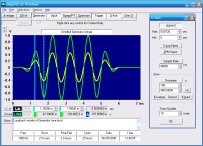
Features:
Oscilloscope
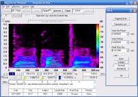
Spectrum Analyzer
8-Channel
Signal Generator
(Absolutely FREE!)
Spectrogram
Pitch Tracker
Pitch-to-MIDI
DaqMusiq Generator
(Free Music... Forever!)
Engine Simulator
LCR Meter
Remote Operation
DC Measurements
True RMS Voltmeter
Sound Level Meter
Frequency Counter
Period
Event
Spectral Event
Temperature
Pressure
MHz Frequencies
Data Logger
Waveform Averager
Histogram
Post-Stimulus Time
Histogram (PSTH)
THD Meter
IMD Meter
Precision Phase Meter
Pulse Meter
Macro System
Multi-Trace Arrays
Trigger Controls
Auto-Calibration
Spectral Peak Track
Spectrum Limit Testing
Direct-to-Disk Recording
Accessibility
Data Logger
Waveform Averager
Histogram
Post-Stimulus Time
Histogram (PSTH)
THD Meter
IMD Meter
Precision Phase Meter
Pulse Meter
Macro System
Multi-Trace Arrays
Trigger Controls
Auto-Calibration
Spectral Peak Track
Spectrum Limit Testing
Direct-to-Disk Recording
Accessibility
Applications:
Frequency response
Distortion measurement
Speech and music
Microphone calibration
Loudspeaker test
Auditory phenomena
Musical instrument tuning
Animal sound
Evoked potentials
Rotating machinery
Automotive
Product test
Contact us about
your application!
Arb_From_Equation Macro Mini-App
- Introduction
- Operation
- Equation Scripts For Included Arbs
- Sine Wave
- Rectified Sines
- Sine Series
- Triangle Wave
- Ramp Wave
- Square Wave
- Pulse Wave
- Full-Scale Pulse Wave
- Tangent Wave
- Half-Tangent Wave
- Gaussian Wave
- Lorentz And Derivative
- Witch Of Agnesi
- Catenary
- Exponential Growth
- Exponential Charge And Decay
- RC Low-Pass Square Wave
- Logarithm
- Square Root
- Power Law
- Ellipses and Circles
- Sinc Function sin(x)/x
- Cosine Window Functions
- Arb_From_Equation Macro Listing
Introduction:
Arb_From_Equation is one of the Macro Examples and Mini-Apps included with Daqarta. It allows you to create an Arb waveform file from an equation that you provide, or modify from one of the included examples.
An Arb file normally holds a single complete cycle of the waveform you want to create, such that when the Daqarta Generator steps through it repeatedly you get a continuous wave at whatever Tone Frequency you have chosen.
However, you are not limited to "normal" continuous waves like sine, triangle, or square; you can use any arbitrary shape that you can define by equations. (See Arb_From_List for another way to create Arb files.) The only requirement is that the equation must produce a series of output values that correspond to increasing X-axis steps: The output can't move backwards in time (or on the screen), so the waveform can't have undercuts. That means, for example, that you can't draw a complete circle on the screen with a single output channel... but you can draw the top half with one channel and the bottom with another. (See the Circle wave discussion, below.)
But producing unusual waveforms is only one use of Arb files. Arbs can also be used as modulator sources for other streams, such as to create waves with arbitrary amplitude or frequency changes. They can serve as lookup tables, such as the Expnote.DAT table of musical note frequency values that can be randomly selected to modulate a stream that creates music. (See the Composer.GEN discussion for an example.)
Operation:
When you run Arb_From_Equation it loads a Generator setup called ArbTest.GEN and fills a Memory Arb (MemArb) with samples computed from the parameters and equation in the macro code. The MemArb is used to create a repeating waveform, with one full cycle displayed on the screen. Note that it may take a few seconds for the full wave to appear; you'll see a "Creating Arb in Memory..." message during this time.
Arb_From_Equation then opens a standard Windows Save As dialog that prompts you for the name of a file to save the Arb as. By default it will be a .DAT file in Daqarta's User_Data folder, but you can navigate elsewhere, or change the file type via the Save as type drop-down control.
You can enter any file name you want, but starting it with Arb_ will make it easier to distinguish from other files in the same folder.
You can hit Cancel if you aren't ready to save the file. Note that at this point the Generator is set to maximum loudness, but muted so you don't have to listen to it. The Y axis thus shows the full-scale output values; the range will be +/-1000 mV (1 V) unless you have done a Full-Scale Range calibration, in which case it will be +/- the calibration value. You can use the cursor readouts to check the values at various points on the waveform.
You can then modify the code and re-run it until you are satisfied with the result.
Setting Arb File Size:
By default, the created Arb will be 16K (16384) samples, the largest size Daqarta supports, for maximum resolution. This size is set via the UK=16 line near the start of the macro code. You can change it to 1, 2, 4, or 8 instead to get smaller files.
Waveform Width Control:
The W=100 line sets the Width of the created wave in percent; assuming that your equation is written to produce one full cycle of the waveform (as in the examples provided), reducing W will compress the waveform into a smaller percentage and fill the remainder with zeros.
For example, the Arb_Sine50.DAT file used W=50 to squeeze one cycle of the sine into the first half of the Arb. If you use this Arb with Tone Freq set to 1000 Hz, for example, you'll get a spectrum with a peak at 1000 (the expected fundamental), plus a peak at 2000 (since the sine wave takes only half the Arb cycle it is twice its frequency), plus components at 3000, 5000, 7000, and all odd multiples of the fundamental. This provides a controlled distortion that adds rich harmonics but is less harsh than other types of distortion such as clipping. This richness is especially noticeable (and pleasant) at low tone frequencies.
You can modify the code to create more than one cycle of the sine wave (or any waveform) in the Width interval. That's especially easy for the sine: Just multiply the contents of the parentheses by the desired number of cycles. For example, the normal sine equation is MemArbV[UA]=K*sin(2*pi*UA/US), so to get UC cycles use MemArbV[UA]=K*sin(UC * 2*pi*UA/US).
Equation Scripts For Included Arbs:
Below are code examples for the Arb files included with Daqarta. You can modify them for your specific needs, or use them as templates to create Arbs from completely different equations.
To use each section below, copy and paste it to replace the section in Arb_From_Equation designated between ;====... comment lines.
Preceding each equation section, the initial part of Arb_From_Equation sets common variables that all equations use.
K=32767, which is the maximum positive output value of the sound card. It is used as a scaling factor so that (for example) a sin() function with a +/-1.00 range will extend over the full range of the sound card.
UN is the number of samples in the Arb, either 1024, 2048, 4096, 8192, or 16384 (default). It is obtained via UN=MemArbV?N after creating the MemArb using MemArbV#N=UK, where UK=16 (or 1, 2, 4, or 8) was given at the start of Arb_From_Equation to set the size.
W is the Width percentage, as described in the Waveform Width Control section above. It defaults to W=100 and can never be greater than 100.
US is set via US=W/100 * UN, giving the number of output samples in the active Width region.
Variable UA starts at 0, and is used as the output sample index.
Each equation section typically consists of one or more WHILE/WEND loops that ultimately step from index 0 to US-1 to create the active output samples. Since the MemArb was filled with all zeros when created, this leaves any remaining samples at 0 if Width is less than 100 percent.
Since each equation section must produce one complete waveform cycle in US samples, each step is 1/US wide and the current step is UA/US.
The Sine Wave equation section below shows how all these variables work together in a typical case.
Note that if you want to create an Arb that is the sum of multiple waves or calculations, you should avoid the seemingly-obvious approach of creating a single full wave over all UN samples of the MemArb, then creating UN additional samples and adding them. Instead, make only a single pass through the MemArb, with each sample being the sum of all the component values at that point. (In other words, the MemArb should only appear on the left side of the expression.)
The reason for this is that a MemArb is standard 16-bit waveform data, whereas the calculations are much higher resolution (32-bit for integers like UN, full 80-bit floating point for variables A-Z). If you compute the waves separately, any roundoff to 16-bit will accumulate.
See the Sine Series section below for the recommended approach.
Sine Wave:
There's never any need for a plain sine wave Arb when using Daqarta with a sound card, since Sine is one of the standard Daqarta Generator wave types.
However, the DaquinOscope macro mini-app uses an Arduino USB board instead of a sound card, and can't use the Generator to create waveforms directly. Instead, it uses the Wave Oscillator function of the DaqPort Arduino code to output a waveform that is first loaded into Arb7 of the Generator and then uploaded to the Arduino as an array of 256 or 1024 8-bit samples. These are then output in a repeating sequence on 8 simultaneous digital output pins for conversion to an analog waveform by means of a simple R-2R ladder DAC. The Wave Oscillator code in DaqPort takes care of stepping through the samples at the proper rate to produce the wave at the desired frequency and phase.
The Arb_Sine.DAT file included with Daqarta was created using the Sine Wave code below. DaquinOscope uses the Port#a7=$(hF0) + "o" or Port#A7=$(hF0) + "O" Bulk Data Write commands to automatically convert the Arb values to the 0-255 range needed, and decimate to 256 or 1024 samples, respectively, before uploading to the Arduino.
Additionally, the Sine Wave code below can be used (with a sound card or DaquinOscope) as the basis for other equations of your own, or for creating "compressed" waveforms with null padding as discussed under Operation - Waveform Width Control, above.
The Arb_Sine50.DAT file included with Daqarta was created using the code section below, with W=50 (near the start of Arb_From_Equation) instead of the default W=100.
;==== Sine Wave ===========================
WHILE.UA=<US
    MemArbV[UA]=K*sin(2*pi*UA/US)  ;Sine wave, scaled to fit in Width
    UA=UA+1
WEND.
;==========================================
Rectified Sines:
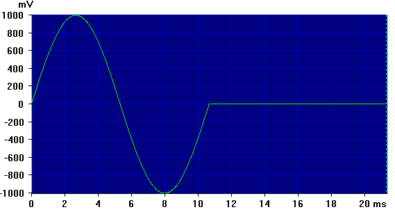
Half-Wave Rectified Sine:
The following code produces a sine wave with only the positive half-cycle present; the negative half is replaced with nulls. This is the waveform created by a single diode rectifier acting upon a sine wave source, as in a simple power supply.
Arb_HalfRectSine.DAT was created with this code.
Note that the code is identical to the normal Sine wave code above, except that the limit of the WHILE loop has been cut in half so that only the first half of the waveform is created.
;==== Half-Wave Rectified Sine ==============
WHILE.UA=<US/2                 ;NOTE the /2 is only difference from Sine
    MemArbV[UA]=K*sin(2*pi*UA/US)  ;Half-cycle of sine
    UA=UA+1
WEND.
;===========================================
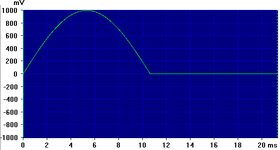
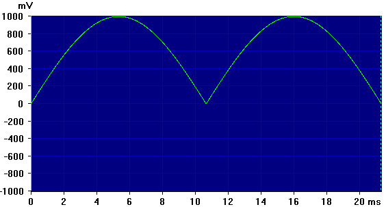
Full-Wave Rectified Sine:
This code is identical to the normal Sine wave code given earlier, except that it uses the {\b abs()} function to take the absolute value. This "flips up" the negative half-cycle to produce a full-wave rectification such as might be found in a power supply using a 4-diode bridge, or 2 diodes with a split-secondary transformer.
Arb_FullRectSine.DAT was created with this code.
;==== Full-Wave Rectified Sine ==============
WHILE.UA=<US
    MemArbV[UA]=abs(K*sin(2*pi*UA/US))
    UA=UA+1
WEND.
;==================================================
Sine Series:
This section includes code for various multi-sine series. The Ramp (Sawtooth), Square, and Triangle Series approximate their namesake waveforms using as many components as you desire. This is controlled by changing a single parameter; 4- and 8-component series examples are shown for Ramp and Square waveforms, but the Triangle series converges so quickly that only a 4-component example is shown.
Note that these "standard waveform" series are also discussed in Making Waves via Sine Wave Synthesis, which uses a separate Generator stream for each sine wave and is limited to 4 terms (although 8 are possible using the Multi-Channel Output Controls, even if you only have a 2-channel sound card.)
Finally, Equal Amplitude Sine Series discusses special test tone complexes, and includes spectra as well as waveform examples.
Note: With all of these series, you use Tone Freq to set the fundamental frequency of the Arb wave. (Even if the fundamental is not actually included, as can be the case in the Equal Amplitude series.) Any harmonics will therefore be multiples of that fundamental, and can easily exceed the Nyquist frequency (half the sample rate) and thus be aliased to lower frequencies. (Try the Aliasing Demonstration to see this in action.)
To prevent this, keep the product of the Tone Freq and the highest harmonic number below half the sample rate. For example, with the 4-component Arb_Sine4Square.DAT discussed in the Sine Square Series section below, the highest harmonic is the 7th. With the default sample rate of 48000 Hz, that means that Tone Freq must be less than 48000 / (2 * 7) = 3428.57 Hz.
But for the 8-component Arb_Sine8Square.DAT the highest harmonic is the 15th, so the maximum Tone Freq would be only 48000 / (2 * 15) = 1600 Hz.
Sine Ramp (Sawtooth) Series:
The Sine Ramp Series approximates a ramp (sawtooth) waveform using a series of sines. The QM parameter sets the number of sine components to be used. The series consists of a fundamental (which would be set by Tone Freq when using the Arb) followed by a series of harmonics: 2nd, 3rd, 4th, etc. The amplitude of each component is scaled according to its reciprocal, so the 2nd harmonic amplitude is half the fundamental, the 3rd harmonic is one-third, and so forth.
We further cut each component in half, including the fundamental, using K/(2*QN) instead of just the K/QN implied above. Otherwise the components add together to be greater than +/-100% at the positive and negative peaks, causing clipping distortion.
Note that some math references (such as Wikipedia) scale by 2/pi, which would be equivalent to K*2/(pi*QN) here. That would work for a 4-component series, but would cause clipping with 5 or more components due to Gibbs phenomenon. (See also the Sine Square Series below.)
The more harmonics that are included, the better the approximation to a ramp. The examples here are for a ramp that starts high and gradually ramps down, which would be equivalent to the normal Ramp Wave using Ramp Rise set to 0. You can easily change that to a ramp that starts low and ramps high (Ramp Rise = 100%) by changing the sign of K in the inner WHILE loop from '+' to '-' as in:
X=X-K/(2*QN)*sin(QN*2*pi*UA/US)
Arb_Sine4Ramp.DAT was created using QM=4 for a 4-component approximation:

Arb_Sine8Ramp.DAT was created using QM=8 for an 8-component approximation:

;==== Sine Ramp Series ====================
QM=4           ;Number of components
WHILE.UA=<US
    QN=1           ;Start with fundamental
    X=0
    WHILE.QN=<(QM+1)
        X=X+K/(2*QN)*sin(QN*2*pi*UA/US)
        QN=QN+1
    WEND.
    MemArbV[UA]=X
    UA=UA+1
WEND.
;==========================================
Sine Square Series:
The Sine Square Series approximates a square waveform using a series of sines. The QM parameter sets the number of sine components to be used. The series consists of a fundamental (which would be set by Tone Freq when using the Arb) followed by a series of odd harmonics only: 3rd, 5th, 7th etc. The amplitude of each component is scaled according to its reciprocal, so the 3rd harmonic amplitude is one-third the fundamental, the 5th harmonic is one-fifth, and so forth.
Note that some math references (such as Wikipedia) also scale by 4/pi, which would be equivalent to K*4/(pi*QN) here. That sets the amplitude of the resultant wave to K, the full-scale range of the sound card. However, the amplitude they are computing is the flat top and bottom of an ideal square wave. But the sine series approximation exhibits an effect known as Gibbs phenomenon, which causes pseudo-"ringing" at each vertical transition. This produces a series of peaks that rise above and below the horizontal parts of the waveform. (See images below.) If the 4/pi scaling set the horizontal to be 100% of the available range, then the Gibbs peaks would attempt to exceed that, and thus cause distortion when they are clipped off.
The more harmonics that are included, the better the approximation to a square. Note, however, that the Gibbs peaks are always present with any finite number of terms.
Arb_Sine4Square.DAT was created using QM=4 for a 4-component approximation. (See this waveform in action with a frequency sweep in the Aliasing Demonstration.) One cycle of the wave looks like this:

Arb_Sine8Square.DAT was created using QM=8 for an 8-component approximation:

;====  Sine Square Series =========
QM=4           ;Number of components
WHILE.UA=<US
    QN=1           ;Start with fundamental
    X=0
    WHILE.QN=<(QM+1)
        X=X+K/(2*QN-1)*sin((2*QN-1)*2*pi*UA/US)
        QN=QN+1
    WEND.
    MemArbV[UA]=X
    UA=UA+1
WEND.
;==================================
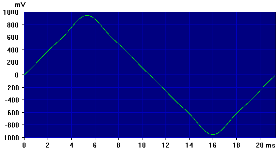
Sine Triangle Series:
The Sine Triangle Series approximates a triangle waveform using a series of sines. The QM parameter sets the number of sine components to be used. The series consists of a fundamental (which would be set by Tone Freq when using the Arb) followed by a series of odd harmonics only: 3rd, 5th, 7th etc. Unlike the Sine Square Series above, each odd harmonic is scaled according to the square of its reciprocal, and the signs of the terms alternate. So the 3rd harmonic is (1/3)^2 or 1/9 of the fundamental and is subtracted, while the 5th harmonic is (1/5)^2 or 1/25 of the fundamental and is added, etc.
The alternating signs of the terms are handled via a factor QI, which starts out as +1 for the fundamental, and is negated for each subsequent harmonic.
The full-scale range value K is adjusted by a scale factor of 8/pi^2 to bring the overall series amplitude close to the original full-scale range.
The more harmonics that are included, the better the approximation to a triangle. However, unlike the above Ramp and Square series, the triangle converges very quickly. Arb_Sine4Triangle.DAT was created using QM=4 for a 4-component approximation. Compared to even the 8-component Ramp and Square series, this is a much better fit to its target waveform:
;====  Sine Triangle Series =========
QM=4           ;Number of components
K=K*8/pi^2     ;Adjust full-scale factor
WHILE.UA=<US   ;Do all sampled
    QN=1           ;Start with fundamental
    X=0            ;Accumulate sample value
    QI=1           ;Alternating sign factor
    WHILE.QN=<(QM+1)   ;Do all harmonics
        X=X+QI*K/(2*QN-1)^2*sin((2*QN-1)*2*pi*UA/US)
        QN=QN+1        ;Next harmonic
        QI=-QI         ;Flip sign for next harmonic
    WEND.          ;Next harmonic
    MemArbV[UA]=X  ;Save sample value
    UA=UA+1        ;Next sample
WEND.
;==================================
Equal-Amplitude Sine Series:
The Equal-Amplitude Sine Series produces QM multiple tones of equal amplitude, which are also equally spaced above an adjustable initial tone. The tones are part of a harmonic series whose fundamental is given by the Tone Freq when using the Arb, but that fundamental is not necessarily included as a component of the series. In fact, the series starts with the QFth harmonic. Furthermore, the spacing of the remainder of the QM tones in the series may be at steps that are some multiple QS of Tone Freq.
This series is typically used to create a particular spectral band of discrete tones for test purposes, as an alternative to band-limited noise testing. Here we give up continuous spectral coverage over the band in exchange for non-random behavior and stable amplitudes, with sharply-defined band edges and component frequencies. You can control the number and density of those components via the QM and QS parameters.
Note that since the QM components have equal amplitudes that start out in-phase and can sum together to large peaks, each of them has been reduced to 1/QM of the full-scale range to prevent clipping. Thus, as you add more components, their levels get smaller. But the resulting levels are still higher than the equivalent with a continuous noise band, for exactly the same reason: The noise band must also guard against clipping at the worst-case instantaneous random waveform peak.
If you have a lot of components and don't really need them to all start at the same phase, it is possible to adjust their individual phases to minimize resulting peak heights, and then boost the overall waveform level above the usual K/QM. See the "Phase Experiments" section of the Missing Fundmental macro mini-app for more details and references.
The Arb_Sine543.DAT example has 5 components (QM=5) starting at 4 times the Tone Freq (QF=4) with a spacing of 3 times the Tone Freq (QS=3). The waveform of a single cycle looks like this:

With a 1 kHz Tone Freq the spectrum has tones at 4, 7, 10, 13, and 16 kHz:

The equal-amplitude series approach was used in the Missing Fundmental macro mini-app, except that had separate signal streams which were individually controlled. The Arb approach is much simpler: You just set Tone Freq to the (missing) fundamental frequency. You can then create bursts or sweeps as desired. As in the mini-app, you can alternate between bursts having different harmonic structures. With the Arb approach you do this using a different Arb in each stream, with burst cycles set the same but with a lag in one of them.
The Arb_Sine521.DAT is a good example of a "missing fundamental" Arb. It has 5 components (QM=5) starting at 2 times the Tone Freq (QF=2) with a spacing equal to the Tone Freq (QS=1). The waveform of a single cycle has this shape:

With a 1 kHz Tone Freq the spectrum has tones at 2, 3, 4, 5, and 6 kHz, all of which are harmonics of the missing 1 kHz fundamental:

;===== Equal-Amplitude Sine Series =====
;Multi-Sine wave with adjustable start and spacing
QM=5           ;Number of components
QF=4           ;Start (* Tone Freq)
QS=3           ;Spacing (* Tone Freq)
WHILE.UA=<US
    QN=1
    X=0
    WHILE.QN=<(QM+1)
        X=X+(K/QM)*sin((QF+(QN-1)*QS)*2*pi*UA/US)
        QN=QN+1
    WEND.
    MemArbV[UA]=X
    UA=UA+1
WEND.
;=======================================
Multiple Sine Wave Harmonics:
This is similar to the above Equal-Amplitude Sine Series, except that it uses only integer harmonics and allows independent amplitudes. It was used to create Arb_Fake_Vowel.DAT, which is an optional waveform for the !Spooky.GEN Sci-Fi Theremin Simulator. It sounds vaguely human in that setup, especially when the pitch is changing between notes.
Arb_Fake_Vowel is also used by Machines.GEN to create a harmonic-rich low-frequency "power hum" for a Halloween "Mad Scientist" laboratory display.
The amplitude of each harmonic is specified in the corresponding element of Buf0: The fundamental is in Buf0[1], the second harmonic in Buf0[2], the third in Buf0[3], etc. QM is then set to the number of components. The code computes all components from 1 to QM, so if you want to skip a harmonic you must set its Buf0[] amplitude to zero.
The following example for Arb_Fake_Vowel.DAT uses the fundamental plus the second and third harmonics. Note that in general the sum of the component amplitudes should not exceed 1.00 to insure there is no clipping, but this example totals 1.15 without clipping.

;==== Multiple Sine Wave Harmonics ========
Buf0[1]=0.5    ;Fundamental amplitude
Buf0[2]=0.25   ;2nd harmonic amplitude
Buf0[3]=0.40   ;3rd harmonic amplitude
QM=3           ;Number of components
WHILE.UA=<US
    QN=1           ;Start with fundamental
    X=0
    WHILE.QN=<(QM+1)
        X=X+K*Buf0[QN]*sin(QN*2*pi*UA/US)
        QN=QN+1
    WEND.
    MemArbV[UA]=X
    UA=UA+1
WEND.
;=================================
Triangle Wave:
As for the Sine Wave code above, there is never any need for a plain triangle wave Arb when using Daqarta with a sound card, since Triangle is one of the standard Daqarta Generator wave types. But the DaquinOscope macro mini-app works with an Arduino USB board instead of a sound card, and uses Arb files uploaded to the Arduino to create waveforms as described under the Sine Wave section.
The Arb_Triangle.DAT file included with Daqarta was created with the Triangle Wave code below to provide a plain triangle wave for this purpose.
Additionally, this code can be used as the basis for other equations of your own, or for creating "compressed" waveforms with null padding as discussed under Operation - Waveform Width Control, above.
Arb_Triangle50.DAT was created with this code, using W=50.
;=== Triangle Wave ========================
US=US/4
S=K / US
WHILE.UA=<US
    MemArbV[UA]=UA * S
    UA=UA+1
WEND.
WHILE.UA=<3*US
    MemArbV[UA]=2*K - (UA * S)
    UA=UA+1
WEND.
WHILE.UA=<4*US
    MemArbV[UA]=(UA * S) - 4 * K
    UA=UA+1
WEND.
;============================================
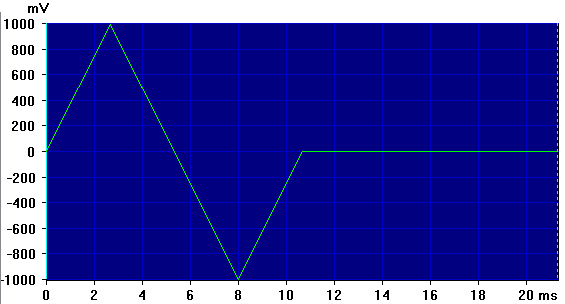
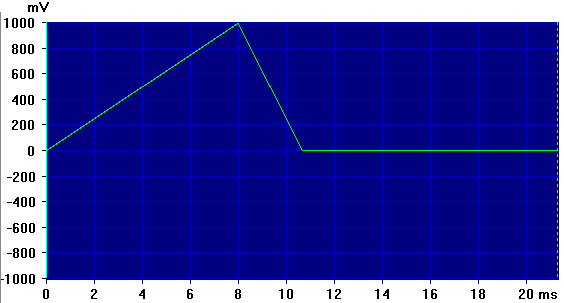
Ramp Wave:
As for the Sine Wave and Triangle Wave code above, there is never any need for a plain ramp wave Arb when using Daqarta with a sound card, since Ramp is one of the standard Daqarta wave types. In fact, the Daqarta Ramp dialog allows easy change of the Ramp Rise (otherwise done via R=75 in the code here), as well as a staircase option and selection of either Phase or Slope modulation types when used with Daqarta's standard Phase Modulation option.
However, the DaquinOscope macro mini-app works with an Arduino USB board instead of a sound card. Its Wave Oscillator function can create waveforms using Arb files uploaded to the Arduino as described under the Sine Wave section.
The Arb_Ramp100.DAT file included with Daqarta was created with R=100 in the Unipolar Ramp Wave code below to provide a plain 0-100% ramp wave for this purpose.
Also, Daqarta's Ramp wave doesn't have a built-in Width option for creating "compressed" waveforms with null padding as discussed under Operation - Waveform Width Control, above.
Arb_75Ramp50.DAT was created with this code, using W=50 together with the default R=75 here.
Note that this wave is unipolar, starting at 0 and rising to 100%, while the standard Generator Ramp wave is bipolar, starting at -100% and rising to +100%. See the Bipolar Ramp Wave code, following, to create compressed bipolar waveforms for sound card use.
;===== Unipolar Ramp Wave =================
R=75                ;Ramp rise percent
S=K / (US * R/100)
WHILE.UA=<US * R/100
    MemArbV[UA]=UA * S
    UA=UA+1
WEND.
UB=UA
S=K / ((1-R/100) * US)
WHILE.UA=<US
    MemArbV[UA]=K - ((UA-UB) * S)
    UA=UA+1
WEND.
;==========================================
The following Bipolar Ramp Wave code was used to create the Arb_Ramp_Bipolar100.DAT file included with Daqarta. Note that R=100 means that with the default W=100 this will create a standard 100% Generator Ramp that starts at -100% and rises to +100%.
;===== Bipolar Ramp Wave ===================
;NOTE that the baseline is -100%, not 0 as
;for Unipolar Ramp Wave.
R=100                ;Ramp rise percent
S=2 * K / (US * R/100)
WHILE.UA=<US * R/100
    MemArbV[UA]=-K + UA * S
    UA=UA+1
WEND.
UB=UA
S=2 * K / ((1-R/100) * US)
WHILE.UA=<US
    MemArbV[UA]=K - ((UA-UB) * S)
    UA=UA+1
WEND.
UB=MemArbV[UA-1]
WHILE.UA=<UN
    MemArbV[UA]=UB
    UA=UA+1
WEND.
;==========================================
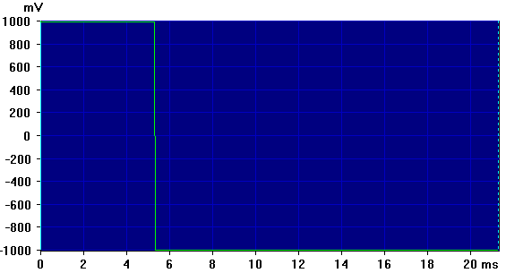
Square Wave:
As for Sine, Triangle, and Ramp above, there's rarely any need for a plain square wave Arb like the included Arb_Square.DAT, since Square is one of the standard Daqarta wave types. And unlike other wave shapes, there is no need for a special Square Arb for the DaquinOscope macro mini-app used with an Arduino board; DaquinOscope standard oscillators (unlike the special Arb-based Wave Oscillators) produce square waves by default.
However, the Square Wave code below can be used as the basis for other equations of your own, or for creating "compressed" waveforms with null padding as discussed under Operation - Waveform Width Control, above.
The Arb_Square50.DAT file included with Daqarta was created using this code, with W=50 (near the start of Arb_From_Equation) instead of the default W=100:
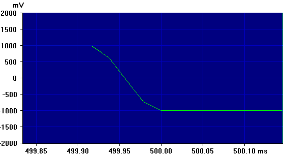
For normal square waves, however, there is another reason to favor the built-in Square over an Arb version: Edge sharpness at low frequencies. The standard Square using Snap mode has edges that always transition in a single sample, although there will be some amount of edge jitter except for particular frequencies.
In Interpolate edge mode, the standard Square has far less jitter, by using softer edge transitions that may take up to 2 samples.
On the other hand, the Arb approach has minimal jitter (at least with the Arb set to Interpolate instead of Round or Step), but at frequencies less than a few Hz the transitions will be spread out over multiple samples. That's because the Arb just does an ordinary overall waveform interpolation, unlike the edge-only Square Interpolate. The image below shows Arb_Square.DAT at a Tone Frequency of 1 Hz, with Trigger Delay and X-Axis eXpand set to show an expanded version of a falling edge. The transition takes 4 samples, although you only see two obvious kinks because the central region is on a straight-line section of the interpolation:
;======= Square Wave ======================
WHILE.UA=<US/2
    MemArbV[UA]=K
    UA=UA+1
WEND.
WHILE.UA=<US
    MemArbV[UA]=-K
    UA=UA+1
WEND.
;===========================================
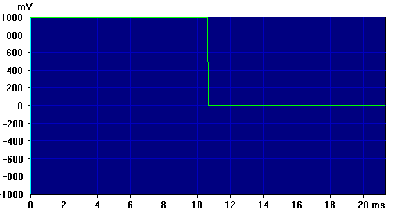
Pulse Wave:
As with the above Square wave, Pulse is one of the standard Daqarta wave types. In fact, the Pulse dialog allows much more control than this simple code, which just produces a single positive pulse whose width is set via the W parameter. (The Pulse dialog allows two separate adjacent pulses with independent widths, levels, and polarities, as well as adjustable baseline and different width/modulation modes.)
Instead, consider this simple code as a starting point for more advanced pulse creation.
Note that if W=100 the pulse will stay high for the full cycle, resulting in a constant full-scale DC waveform. Since standard sound cards block DC, there will be no output at all. (True, you could use this to provide a DC modulation source, but you can do that simply by using the built-in Sine wave with Phase set to 90 degrees.)
Arb_Pulse50.DAT was created with this code, using W=50. This gives a positive-only square wave output. Again, since sound cards are AC-coupled, this is only useful as a modulation source. However, the DaquinOscope macro mini-app uses an inexpensive Arduino board to acquire DC data, and has an optional wavetable oscillator that produce arbitrary output waveforms. This or the following full-scale pulse will indeed produce DC pulses.
;======= Pulse Wave ========================
;NOTE that if W=100 this just gives constant K level
WHILE.UA=<US
    MemArbV[UA]=K
    UA=UA+1
WEND.
;===========================================
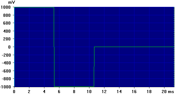
Full-Scale Pulse Wave:
This is just like the above Pulse Wave, except that instead of a full-scale positive pulse that returns to a baseline of zero, this returns to full-scale negative. Also as above, this could have been done with the Pulse that is one of the standard Daqarta wave types, just by adjusting the zero level in the Pulse dialog, so consider this as a code example.
Likewise, if W=100 the pulse will stay high for the full cycle, resulting in a constant full-scale DC waveform.
Arb_FSPulse25.DAT was created with this code, using W=25 to produce a pulse that is high for 25% of the cycle.
;======= FS Pulse Wave ======================
;NOTE that if W=100 this just gives constant K level
WHILE.UA=<US
    MemArbV[UA]=K
    UA=UA+1
WEND.
WHILE.UA=<UN
    MemArbV[UA]=-K
    UA=UA+1
WEND.
;============================================
Tangent Wave:
This code was used to create Arb_Tan.DAT, which is a plot of the tangent function over one full circle. Note that the tangent is discontinuous at pi/2 and 3*pi/2 radians, where it goes from positive to negative infinity. Since this would be awkward to try to reproduce with a sound card that is limited to +/-32767, the waveform has been scaled down by a factor of 128. Feel free to experiment with other scale factors depending on your needs.
;======= Tan Wave ===========================
;NOTE that this has two peaks per cycle
K=K/128            ;Reduce scale factor for less peak clipping
WHILE.UA=<US
    MemArbV[UA]=K*tan(2*pi*UA/US)
    UA=UA+1
WEND.
;============================================
Half-Tangent Wave:
As above, but Arb_HalfTan.DAT produced with this code only covers half of a full circle by using tan(pi*UA/US) instead of tan(2*pi*UA/US). This give a single biphasic +/- full-scale spike at the center of the waveform (pi radians), instead of narrower spikes at pi/2 and 3*pi/2.
;======= Half Tan Wave ===========================
;As above, but single peak per cycle
K=K/128            ;Reduce scale factor for less peak clipping
WHILE.UA=<US
    MemArbV[UA]=K*tan(pi*UA/US)
    UA=UA+1
WEND.
;============================================
Gaussian Wave:
The Gaussian curve describes what is known as a 'normal' distribution in statistics. It is the standard example of a "bell-shaped curve". The code included here is for a 'standardized' version, in which the central peak is always unity (full scale here). The standard deviation D adjusts the width of the peak, with the default 1.00 producing tails that are 0.0072 (236 counts out of the full-scale 32767 counts). This was used to create the included Arb_Gauss.DAT file.
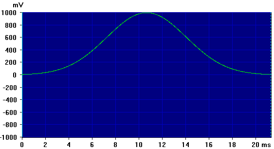
If you set D=0.70 instead, the tails will be 0.00003, or one count out of 32767.
The width of the peak at half-maximum (FWHM) as a fraction of the total width is found by FWHM = 0.375 * D.
;======= Gaussian ===========
;With D=1.00, tails = 0.0072
;With D=0.70, tails = 0.00003
;Central peak always 1.000 (Full scale)
M=0                        ;Mean = 0
D=1.00                     ;Standard Deviation
D=D / (2 * pi)             ;Working value
C=sqrt(2 * pi)             ;0.3989
K=K * C
WHILE.UA=<US
    X=(UA-(US/2)) / US
    Z=(X - M) / D
    MemArbV[UA]=K * exp(-Z^2 / 2) / C
    UA=UA+1
WEND.
;==============================
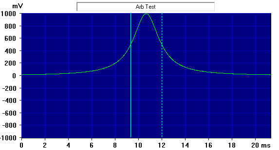
Lorentz And Derivative:
Lorentz:
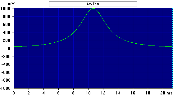
The Lorentz or Lorentzian distribution is also known as a Cauchy distribution. It is similar to a Gaussian in that it is a "bell-shaped curve" tapering from a central peak. The simplified equation is Y=1/(X^2 + 1), but we'd like to control the width of the peak, the way standard deviation does for the Gaussian.
We use P as the width of the peak at half-maximum height (FWHM), and working variable G=P / 2. The revised simplified equation then becomes Y=G / (X^2 + G^2). Note, however, that this formulation is not normalized: The peak height changes with width. The code below keeps a constant full-scale height using Y=G^2 / (X^2 + G^2).
Arb_Lorentz_8th.DAT was created with the default P=0.125, which gives a width that is 1/8 of the full Arb cycle:
;======= Lorentz ================
P=0.125             ;Width of peak at half height
G=P / 2
WHILE.UA=<US
    X=(UA-US/2)/US
    MemArbV[UA]=K * G^2 / (X^2 + G^2)
    UA=UA+1
WEND.
;==============================
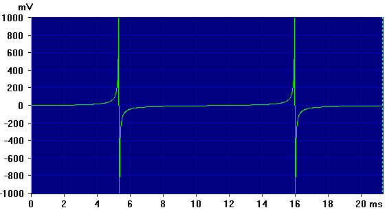
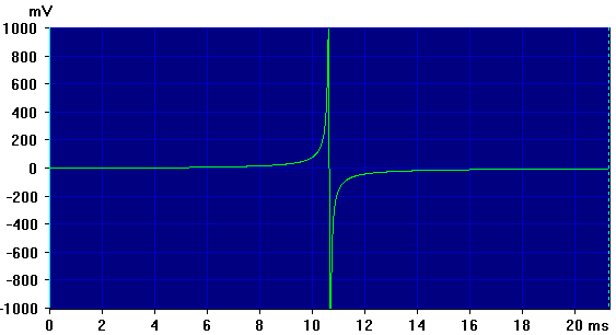
D_Lorentz:
The derivative of the Lorentz function is a biphasic pulse. The 'standard' equation is Y=-2 * X / (X^2 + 1)^2. Using the same width control P from the above raw Lorentz, along with working variable G=P / 2, the derivative would be Y=-2 * X / (X^2 + G^2)^2. However, as with the raw Lorentz, we also normalize to keep constant full-scale peak heights. The normalized formula is Y=-2 * X * G^3 / (X^2 + G^2)^2.
Note that although the peak heights are normalized, this does not automatically provide for a useful repeating waveform. The problem is that unless the width is kept very small (P=0.017 or less), the starting amplitude and the ending amplitude are different, which would result in an abrupt step at the end of each cycle. Below are plots for various P values:
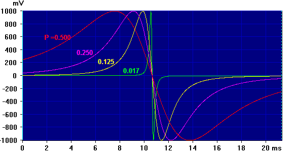
The Arb_D_Lorentz.DAT file is shown as the green curve for P=0.017. The tails are both zero, so there is no step. If the full-scale output range is +/-1000 mV, the steps for the other P values are:
      P         Step, +/-mV
    0.500       247
    0.250       42.6
    0.125       5.8
    0.017       0.0
;======= D-Lorentz ================
P=0.017         ;Width of raw Lorentz peak
G=P/2
K=K / 0.6495    ;Scaling for full-scale peaks
WHILE.UA=<US
    X=(UA-US/2)/US
    MemArbV[UA]=K * (-2 * X) * G^3 / (X^2 + G^2)^2
    UA=UA+1
WEND.
;==============================
Witch Of Agnesi:
This is another "bell-shaped curve" like the Gaussian and Lorentz. According to Wikipedia and Wolfram, it was described by Maria Agnesi in a 1748 book that is the oldest surviving mathematical work by a woman. The "witch" in the name comes from a later mis-translation of averisera, the Italian for a "turning sine curve" into avversiera, a female devil, and later simply "witch".
The P parameter controls the width of the curve, as a fraction of the full cycle width. This is the width of the peak at half-maximum height (FWHM).
Arb_Agnesi.DAT was created with the default P=0.05:
;==== Witch of Agnesi ====================
P=0.05
A=P * 2
K=K / (2 * A)
WHILE.UA=<US
    X=2 * UA/US - 1
    MemArbV[UA]=K * 8 * A^3 / (X^2 + 4*A^2)
    UA=UA+1
WEND.
;==========================================
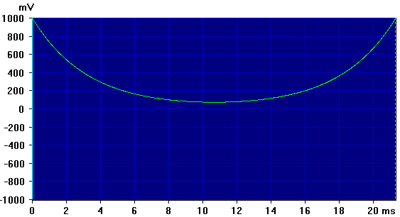
Catenary Curve:
A catenary curve describes the shape of an idealized rope or chain hanging freely between two end points, with no other load than its own weight. The value of A used here is selected such that the ends are at full scale. This was used to create the included Arb_Catenary.DAT file.
;======= Catenary ===========
A=0.0765                   ;Selected to get full scale in 16K samples
WHILE.UA=<US
    X=0.5 * (UA-US/2)/US
    MemArbV[UA]=K*A*cosh(X / A)
    UA=UA+1
WEND.
;==============================
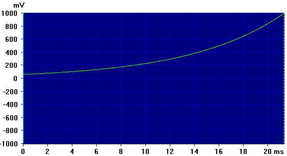
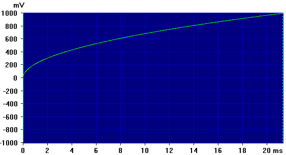
Exponential Growth:
The Exponential Growth Arb Arb_Exp_Growth.DAT plots the growth of something whose growth rate is proportional to the current value - the greater it is, the faster the rise. Here we use B as the growth factor and A as the number of time constants to be plotted, where one time constant is the time for the output to increase by the factor B. The time constant is thus 1/A.
The default code uses B=2 and A=4, which could represent a plot of 4 doublings (4 time constants) of a bacterial colony:
;===========Exponential Growth ===============
A=4                    ;Include 4 time-constants in Arb
B=2                    ;Growth factor: Output multiplies by B in 1/A time
K=K / (B^A)            ;Initial value to reach full scale at end
WHILE.UA=<US
    X=UA/US
    MemArbV[UA]=K * B^(A * X)
    UA=UA+1
WEND.
;==============================
Exponential Charge And Decay:
Exponential Charge:

The Exponential Charge Arb Arb_Exp_Charge.DAT is the shape of the voltage-versus-time curve for a capacitor C being charged through a resistor R, where the charging voltage is the full-scale range of the sound card K = 32767. The product of R * C has units of seconds and is known as the time constant, which we'll call T here. This is the time at which the capacitor reaches 63.2% of the maximum voltage. (That's 1 - 1/e or 0.6321056.)
In the code below, we use A to specify how many of these T time constants will be included in the Arb. We don't use T directly there.
To use the Arb to model real resistors and capacitors, you need to consider the Tone Frequency used by the Arb. That determines the period of Arb model of the charging curve. Arb_From_Equation sets this as:
L.0.ToneFreq=SmplRate / 1024
This spreads the curve over one full waveform screen of 1024 samples, to aid in evaluating the Arb being created. But you are not limited to that when you later use the created Arb for your own applications. The time for one period of the Arb (A time constants) will be 1 / ToneFreq, so the time T for one time constant will be:
T = R * C = 1 / (A * ToneFreq).
Substituting, we can solve solve for R, C, A, or ToneFreq:
R = 1 / (R * A * ToneFreq)
C = 1 / (C * A * ToneFreq)
A = 1 / (R * C * ToneFreq)
ToneFreq = 1 / (R * C * A)
;======= Exponential Charge ============
A=4                    ;Include 4 time-constants in Arb
WHILE.UA=<US
    X=UA/US
    MemArbV[UA]=K * (1 - exp(-A * X))
    UA=UA+1
WEND.
;==============================
Exponential Decay:
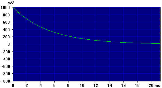
Conversely, the Exponential Decay Arb Arb_Exp_Decay.DAT is the shape of the voltage-versus-time curve for a capacitor C being discharged through a resistor R, from an initial starting voltage equal to the full-scale range of the sound card. All the same time constant math applies.
;======= Exponential Decay =============
A=4                    ;Include 4 time-constants in Arb
WHILE.UA=<US
    X=UA/US
    MemArbV[UA]=K * exp(-A * X)
    UA=UA+1
WEND.
;==============================
RC Low-Pass Square Wave:
Arb_RC_LowPass_Square.DAT combines the above Exponential Charge and Exponential Decay to simulate a square wave passed through a simple RC lowpass filter.
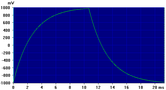
Note that this code is for a bipolar square wave that is symmetrical about zero volts, such as the normal Generator Square Wave option. This is slightly more complex than a positive-only square wave, but in either case we need more than a simple concatenation of Charge and Decay code.
To understand the issue, consider simulating a positive-only square. We start with the Charge code for half the cycle, followed by the Decay code for the remainder. But note that the Charge curve starts at zero volts but doesn't reach the full-scale value; it only approaches it as you increase the number of time constants. Conversely, the Decay curve starts at full scale but doesn't reach zero. The simple code concatenation would thus produce an abrupt step up at the start of the Decay phase, and an abrupt step down to zero at the start of the following Charge.
To correct for this, we need to shift each phase by an amount that depends on its end value, which we must pre-compute so we can include the shift in each sample. For the bipolar square we must also double the range and shift it down so half is negative.
Note that here A is the number of time constants in each phase of the square wave.
;======= RC Low-Pass Square Wave =============
A=4                    ;Include 4 time-constants in each phase
D=K * (1 - exp(-A))    ;Precompute end of Charge phase (where X=1)
Q=K - D                ;Difference from full-scale K
A=A * 2                ;Double A to cover half cycle
WHILE.UA=<US/2
    X=UA/US
    V=K * (1 - exp(-A * X))
    MemArbV[UA]=2 * V - D
    UA=UA+1
WEND.

UA=0
D=D + 2 * Q
WHILE.UA=<US/2
    X=UA/US
    V=K * exp(-A * X)
    MemArbV[UA+US/2]=2 * V - D
    UA=UA+1
WEND.
;==============================
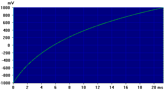
Logarithm:
Arb_Log.DAT is the plot of a logarithmic curve that has been scaled and offset so that it runs from negative full scale to positive full scale.
The raw equation would look something like Y=ln(X). To facilitate the scaling and offset calculations, we first rewrite it to Y=K * (1 + ln(X)). We then replace X with X=A * UA/US + B, where US is the total number of sample points in the Arb, and UA is the sample index which runs from 0 to US-1.
The sound card full-scale value is K=32767, and we want the 0th point to be -K or -32767. When UA = 0, X=A * UA/US + B becomes X=B, so we can insert that into Y=K * (1 + ln(X)) to get Y=K * (1 + ln(B)). Since we want the result to be -K here, we can set Y=-K and get -K=K * (1 + ln(B)). Dividing both sides by K gives -1=1 + ln(B), thus ln(B)=-2, hence B=exp(-2).
To find the value for A we use the condition when UA=(US-1) and set that to give an output of +K. K=K * (1 + ln(X)) then becomes 1=1 + ln(X) and ln(X)=0. Since X=A * UA/US + B, we get ln(A * UA/US + B) = 0. But we know that 0 is the log of 1, so we can remove the logarithm to get A * UA/US + B = 1 and solve for A when UA=US-1 to get A=(1 - B) * US / (US-1).
We solve for B and A outside the main loop, since these don't change during the Arb calculation.
;======= Log =============
B=exp(-2)                  ;Constant to set 0th point to -K
A=(1 - B) * US / (US-1)    ;Constant to set final point to +K
WHILE.UA=<US
    X=A * UA/US + B        ;Scaling and offset to get +/-FS range
    MemArbV[UA]=K * (1 + ln(X))
    UA=UA+1
WEND.
;=========================
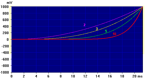
Power Law:
This code creates the curve of Y=X^P as X runs from 0 to 1, scaled so that the output runs from 0 to K, the sound card full-scale value. The code below shows P=2 to give a square law, but any positive value will work, including fractions. Using P=0.5 will give the same curve as Arb_SquareRoot.DAT in the next subtopic.
Included waveforms are Arb_Power_2.DAT, Arb_Power_3.DAT, Arb_Power_5.DAT, and Arb_Power_10.DAT for powers 2, 3, 5, and 10. The image below shows all of these superimposed for comparison:
;===== Power Law ======================
P=2                    ;Power, may be decimal
P=abs(P)               ;Not negative
WHILE.UA=<US           ;Compute 0 to US points
    X=UA / (US - 1)        ;Scaling to get FS at peak
    MemArb0[UA]=K * X^P    ;Compute and save
    UA=UA+1                ;Next sample
WEND.
;========================================
Square Root:
Arb_SquareRoot.DAT is the plot of Y=sqrt(X) as X runs from 0 to 1, scaled so that the output runs from 0 to K, the sound card full-scale value.
;======= Square Root =============
WHILE.UA=<US
    X=UA/US
    MemArbV[UA]=K * sqrt(X)
    UA=UA+1
WEND.
;==============================
Ellipses And Circles:
Half Ellipse (Half Circle):
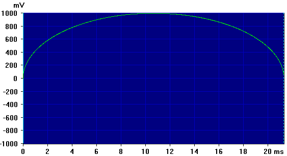
Arb_Half_Ellipse.DAT is the plot of the top half of an ellipse or a circle; the appearance depends on the Y-axis magnification and the tone frequency the Arb is run at. At full-scale magnification with one Arb cycle (one half of the ellipse) on the screen, as shown when you run this code in Arb_From_Equation, you see a half-ellipse that looks like a slightly squashed circle. If you double the tone frequency you see two half-circles (assuming your monitor has square pixels).
;======= Half Ellipse (Half Circle) =============
WHILE.UA=<US
    X=2 *(UA-US/2)/US
    MemArbV[UA]=K * sqrt(1 - X^2)
    UA=UA+1
WEND.
;=============================
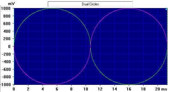
Alternating Half Ellipse And Dual Circles
Arb_Alt_Half_Ellipse.DAT alternates the top (positive) half of an ellipse or circle with the bottom (negative) half in each full cycle of the Arb. It looks somewhat like a deformed sine wave. However, when the same wave is output on both Left and Right channels, but with one channel inverted, you see two adjacent full circles. The Circles.GEN generator setup has been created to do exactly this.
If you cut the screen magnification in half (PgDn key) you will see two ellipses. If you then double the Left and Right tone frequencies from 46.875 to 93.75 Hz you will see 4 circles.
;======= Alternating Half Ellipse ("Circle" Wave)===
WHILE.UA=<US/2
    X=4 * (UA-US/4)/US
    MemArbV[UA]=K * sqrt(1 - X^2)
    MemArbV[UA+US/2]=-K * sqrt(1 - X^2)
    UA=UA+1
WEND.
;==============================
Sinc Function sin(x)/x:
The sinc function looks like a sinusoid that decays on either side of a central peak, somewhat like a "ringing" bell-shaped curve:
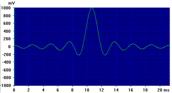
In the code supplied here, parameter F controls the "frequency" of the sinusoid; it is essentially the number of half-cycles (positive or negative peaks) in each half of the waveform, counting the central peak.
Note that if F is an integer, the waveform will start at 0 and end at 0. However, since the waveform is mirrored about the center, that also means that when the waveform repeats it is likewise mirrored about its ends. For example, if the start is at 0 with a positive slope, the end will have a negative slope down to 0 that will not "splice" smoothly with the next start rising up from 0.
To get a smooth splice-free wave, you must set F to halfway between two integers. The image above (which is also the Arb_Sinc85.DAT waveform) used the default F=8.5. Note that it starts and ends at a positive peak, instead of a zero, so it will splice perfectly.
;=== Sinc Function ===============================
F=8.5                      ;"Frequency"
WHILE.UA=<US/2
    X=F*2*pi*UA/US
    Y=K*sin(X) / X
    MemArbV[UA+US/2]=Y         ;Fill from center up
    MemArbV[US/2-UA]=Y         ;Fill from center down
    UA=UA+1
WEND.
MemArbV[US/2]=K            ;Center = 1.00
;============================================
Cosine Window Functions:
Here we include code to create Arbs of several common window functions, the same ones used by Daqarta to reduce spectral leakage. They all use the same code, but with different parameter values. (Note that in the plot below all three Blackman curves nearly overlay, so at this scale they appear as a single yellow line.)

Hann (Haversine):
Arb_Hann.DAT was created with the code below:
;===============================================
A=0.5              ;Hann (same as Haversine)
B=0.5
C=0

;General Cosine Window:
WHILE.UA=<US
    X=2 * pi * (UA / (US-1))            ;Center the window in Width
    Y=A - B * cos(X) + C * cos(2 * X)
    Y=Y * K
    MemArbV[UA]=Y
    UA=UA+1
WEND.
;===============================================
Hamming:
Arb_Hamming.DAT was created using the following parameters in the above Cosine Window code:
A=0.54             ;Hamming
B=0.46
C=0
Blackman:
Arb_Blackman.DAT was created using the following parameters in the above Cosine Window code:
A=0.42             ;Blackman
B=0.5
C=0.08
Blackman Exact:
Arb_BkmExact.DAT was created using the following parameters in the above Cosine Window code:
A=0.42659071       ;Blackman Exact
B=0.49656062
C=0.07684867
Blackman-Harris:
Arb_BkmHarris.DAT was created using the following parameters in the above Cosine Window code:
A=0.42323          ;Blackman-Harris
B=0.49755
C=0.07922
Flat-Top:
Arb_FlatTop.DAT was created using the following parameters in the above Cosine Window code:
A=0.2810639        ;Flat-Top
B=0.5208972
C=0.1980399
Arb_From_Equation Macro Listing:
;<Help=H491F
UK=16                  ;16K = 16384 samples (1,2,4,8,16 allowed)
W=100                  ;Waveform uses 100% Width of above
W=abs(W)               ;Must be positive
IF.W=>100              ;Can't use more than 100%
    W=100
ENDIF.

Spect=0                ;Spectrum off
Sgram=0                ;Spectrogram off
Xpand=0                ;Show full horzontal range
TraceMag=0             ;Show full vertical range
Msg="Creating Arb in Memory..."
A.LoadGEN="ArbTest"    ;GEN to hold MemArb, muted Full Scale range
Ch=0                   ;Use MemArb0
MemArbV#X=0            ;Remove existing MemArb or Arb, if any
MemArbV#N=UK           ;Create 1, 2, 4, 8, or 16K MemArb
L.0.Arb0=1             ;Set output active
UN=MemArbV?N           ;Get size in samples
K=32767                ;Sound card +/- full-scale value

Decimate=0             ;Decimate OFF
L.0.ToneFreq=SmplRate / 1024    ;One cycle on screen
US=W/100 * UN          ;Samples in active Width section
UA=0                   ;MemArb sample index

;==== Sine Wave === (REPLACE as desired) ====================
WHILE.UA=<US
    MemArbV[UA]=K*sin(2*pi*UA/US)  ;Sine wave, scaled to fit in Width
    UA=UA+1
WEND.
;============================================================

WaitSecs=3         ;Wait for sound card output buffer fill
Msg=
MemArbV="<Save:"
See also Memory Arbs (MemArb0-7), Arb Files as Controllers, MemArb_To_File Macro, Wave Dialog, Arb Wave.
- Back to MemArb_To_File Macro
- Ahead to Arb Files as Controllers
- Daqarta Help Contents
- Daqarta Help Index
- Daqarta Downloads
- Daqarta Home Page
- Purchase Daqarta
Questions? Comments? Contact us!
We respond to ALL inquiries, typically within 24 hrs.INTERSTELLAR RESEARCH:
Over 35 Years of Innovative Instrumentation
© Copyright 2007 - 2023 by Interstellar Research
All rights reserved