Software for Windows
Science with your Sound Card!
Features:
Oscilloscope
Spectrum Analyzer
8-Channel
Signal Generator
(Absolutely FREE!)
Spectrogram
Pitch Tracker
Pitch-to-MIDI
DaqMusiq Generator
(Free Music... Forever!)
Engine Simulator
LCR Meter
Remote Operation
DC Measurements
True RMS Voltmeter
Sound Level Meter
Frequency Counter
Period
Event
Spectral Event
Temperature
Pressure
MHz Frequencies
Data Logger
Waveform Averager
Histogram
Post-Stimulus Time
Histogram (PSTH)
THD Meter
IMD Meter
Precision Phase Meter
Pulse Meter
Macro System
Multi-Trace Arrays
Trigger Controls
Auto-Calibration
Spectral Peak Track
Spectrum Limit Testing
Direct-to-Disk Recording
Accessibility
Data Logger
Waveform Averager
Histogram
Post-Stimulus Time
Histogram (PSTH)
THD Meter
IMD Meter
Precision Phase Meter
Pulse Meter
Macro System
Multi-Trace Arrays
Trigger Controls
Auto-Calibration
Spectral Peak Track
Spectrum Limit Testing
Direct-to-Disk Recording
Accessibility
Applications:
Frequency response
Distortion measurement
Speech and music
Microphone calibration
Loudspeaker test
Auditory phenomena
Musical instrument tuning
Animal sound
Evoked potentials
Rotating machinery
Automotive
Product test
Contact us about
your application!
Macro Array Math Operations
- Command Summary
- Basic Array Math
- Complex Number Array Math
- Logarithmic and Exponential Operations
- Powers
- Array Index As Value
- Interpolation
- Integrals and Derivatives
- Total Integration (Summation) and Dot Products
- Peak Functions
- Index Range Cropping
Command Summary:
 Basic Array Math:
Buf0="<+(K)"       Add K to each Buf0 element
Buf0="<-(K)"       Subtract K
Buf0="<*(K)"       Multiply by K
Buf0="</(K)"       Divide by K
Buf0="<\(K)"       Buf0 = K / Buf0
Buf0="<~(K)"       Buf0 = K - Buf0

Buf0="<+B1"        Buf0 + Buf1
Buf0="<-B1"        Buf0 - Buf1
Buf0="<*B1"        Buf0 * Buf1
Buf0="</B1"        Buf0 / Buf1
Buf0="<\B1"        Buf0 = Buf1 / Buf0
Buf0="<~B1"        Buf0 = Buf1 - Buf0
Buf0="<|"          Absolute value

 Complex Number Array Math:
Buf0="<c+(A,B)"    Add complex A + jB to Buf0
Buf0="<c+B1"       Add complex Buf1
Buf0="<c-(A,B)"    Subtract complex A + jB
Buf0="<c-B1"       Subtract complex Buf1
Buf0="<c~(A,B)"    Buf0 = A + jB - complex Buf0
Buf0="<c~B1"       Buf0 = complex Buf1 - Buf0
Buf0="<c*(A,B)"    Complex Buf0 * A + jB
Buf0="<c*B1"       Complex Buf0 * Buf1
Buf0="<c/(A,B)"    Complex Buf0 / A + jB
Buf0="<c/B1"       Complex Buf0 / Buf1
Buf0="<c\(A,B)"    Buf0 = A + jB / complex Buf0
Buf0="<c\B1"       Buf0 = complex Buf1 / Buf0
Buf0="<c**"        Complex conjugate of Buf0

 Logarithmic and Exponential Operations:
Buf0="<L(K)"       K * log2(Buf0)
Buf0="<l(K)"       As above, but only elements 0-511
Buf0="<E(K)"       2^(K * Buf0)
Buf0="<e(K)"       As above, but only elements 0-511

 Powers:
Buf0="<*B0"        Square Buf0
(See the  Powers topic for other powers)

 Array Index As Value:
Buf0="<=#"         Buf0 = 0, 1, 2, ... 1023
Buf0="<c=#"        Buf0 = (0,0), (1,1), (2,2), ... (511,511)
Buf0="<c=#r"       Buf0 = (0,?), (1,?), (2,?), ... (511,?)
Buf0="<c=#i"       Buf0 = (?,0), (?,1), (?,2), ... (?,511)

 Interpolation:
Y=Buf0?i[X]        Y = interpolated value for index X.nnn

 Integrals and Derivatives:
Buf0="<I"          Integral of Buf0 (cumulative summation)
Buf0="<D"          Derivative of Buf0 (incremental difference)

 Total Integration (Summation) and Dot Products:
X=Buf0?U           X = sum of all Buf0 elements

 Peak Functions:
P=Buf0?p           P = most-positive element of Buf0
N=Buf0?n           N = most-negative element of Buf0
P=pkB(N)           P = most-positive element of BufN
P=pkb(N)           As above but only elements 0-511
UI=Posn?p          UI = index of any of the above

 Index Range Cropping:
Buf0="<o(A,B)"     Nulls Buf0 except between indexes A to B, inclusive
Buf0="<o(B,A)"     Nulls Buf0 only between indexes A to B, inclusive
Basic Array Math:
Buf0="<+(K)" adds the current value of K to each element of Buf0. K can be any constant, variable, control value, or expression; parentheses around it are mandatory.
Buf0="<+B1" adds each element of Buf1 to the corresponding element of Buf0.
In this and any buffer command that requires a source (right side) buffer number you can use an expression for the buffer by enclosing it in parentheses, as in Buf0="<+B(X+Y)". Be careful not to confuse this with the above (K) addition, which lacks the B before the parentheses.
Subtraction, multiplication, and division work just like the above addition example, using -, *, and / operators instead of +. Addition and subtraction overflows are "clipped" to the maximum positive or negative values that fit in the data format...just under +/-2^31 (-2147483648 to +2147483647.999999999). Multiplication overflow or division by zero always yield the maximum value, with the correct sign.
Exception: Zero divided by zero gives a unity result by default. You can change this behavior to give zero or maximum negative via the Posn#Z command.
Use \ instead of / for "reverse division". Buf0="<\(K)" replaces each element of Buf0 with K / Buf0. This yields the reciprocal of each element if K=1. Similarly, Buf0="<\B1" replaces each element of Buf0 with Buf1 / Buf0. Reverse division is like normal division with respect to division by zero, and also defaults to unity for zero divided by zero unless set otherwise via Posn#Z. (However, if K=0 then the array is simply filled with zeros and no division is perfomed.)
Use ~ (tilde) instead of - to perform "reverse subtraction". Buf0="<~(K)" replaces each element of Buf0 with K minus the original element value. This yields negation if K=0. Similarly, Buf0="<~B1" replaces each element of Buf0 with Buf1 - Buf0.
Buf0="<|" takes the absolute value of each element of Buf0.
Complex Number Array Math:
Complex numbers have separate real and imaginary components, usually given as a pair with the real component first. This is sometimes denoted by Re,Im. The typical math expression is usually of the form A + jB or A + iB, where A is the value of the real component, B is the value of the imaginary component, and j or i is the square root of -1. (Mathematicians typically use i, while engineers use j to prevent confusion with current, which is usually denoted by i.)
A and B values may be positive or negative.
As described under Macro Array Spectrum Operations, the 1024-value macro arrays Buf0-Buf7 can be utilized as 512 complex pairs, with the even elements holding real values and the odd elements holding imaginary values. That format is used for raw spectral data from Daqarta's Fast Fourier Transform (FFT) operations.
Besides copying complex spectral data from the sound card channels using (for example) Buf0="<=S1" to copy from the Right In spectrum channel 1, you can also copy from another array via Buf0="<c=B1", or fill an array with a complex constant via Buf0="<c=(A,B)".
In addition, there are several ways to fill an array with index values, which can then be scaled by complex multiplication to get complex values proportional to array index. See the Array Index As Value topic, below.
Given two complex pairs A + jB and C + jD, there are special rules for the basic math operations discussed above, which can likewise be applied to entire arrays with single commands.
Addition:
The longhand way to add two complex values A + jB and C + jD:
(A + jB) + (C + jD) = (A+C) + j(B+D)
Adding complex value A + jB to array Buf0:
Buf0="<c+(A,B)"
Adding complex array Buf1 to Buf0:
Buf0="<c+B1"
Subtraction:
The longhand way to subtract two complex values A + jB and C + jD:
(A + jB) - (C + jD) = (A-C) + j(B-D)
Subtracting complex value A + jB from array Buf0:
Buf0="<c-(A,B)"
Subtracting complex array Buf1 from Buf0:
Buf0="<c-B1"
Reverse subtraction to replace each element of Buf0 with A + jB minus the original value:
Buf0="<c~(A,B)"
Reverse subtraction to replace each element of Buf0 with Buf1 - Buf0.
Buf0="<c~B1"
Multiplication:
The longhand way to multiply complex values A + jB times C + jD:
(A + jB) * (C + jD) = (AC-BD) + j(BC+AD)
Note that if one term is set to zero the result is the same as a simple multiply that operates on each term, Re and Im alike. For example, if D = 0:
    (A + jB) * (C + j0) = (AC - B0) + j(BC + A0)
                            = (AC + jBC)
Multiplying complex value A + jB times each complex element in array Buf0:
Buf0="<c*(A,B)"
Multiplying complex array Buf0 times Buf1:
Buf0="<c*B1"
Division:
The longhand way to divide complex value A + jB by C + jD:
                            AC+BD       BC-AD
    (A + jB) / (C + jD) =  ------- + j -------
                           C^2+D^2     C^2+D^2
Dividing each element in Buf0 by the complex value A + jB:
Buf0="<c/(A,B)"
Dividing complex array Buf0 by Buf1:
Buf0="<c/B1"
Reverse division to replace each element in Buf0 with A + jB divided by the original value:
Buf0="<c\(A,B)"
Reverse division to replace each element in Buf0 with Buf1 / Buf0
Buf0="<c\B1"
Complex Conjugate:
The conjugate of complex number is found by simply negating the imaginary portion. For example, if the original value is 7 + j3 the conjugate is 7 - j3. If you apply the conjugate operation a second time, you get back the original value. To take the conjugate of all the complex values in buffer Buf0, use:
Buf0="<c**"
One use for the complex conjugate is to null all the imaginary terms in an array. If you add a complex number and its conjugate, as in (A + jB) + (A - jB), the result is 2*A + j0: The imaginary term is cancelled while the real term is doubled. Then you can multiply by 1/2 to get only the original real. Assuming you want to do this to an array in Buf0:
    Buf1="<c=B0"           ;Copy to Buf1 (A + jB
    Buf1="<c**"            ;Complex conjugate (A - jB)
    Buf0="<c+B1"           ;Add to original (2*A + j0)
    Buf0="<c*(0.5,0)"      ;Original Re values (A + j0)
Note that the final step used a complex multiply by (0.5,0) but a normal Buf0="<*(0.5,)" multiply would work as well (and be slightly faster) since it would simply take half of every term, where half of the zero imaginary term is still zero.
Conversely, you can cancel all the real terms and keep only the imaginary by subtracting the conjugate from the original:
    Buf1="<c=B0"           ;Copy to Buf1 (A + jB)
    Buf1="<c**"            ;Complex conjugate (A - jB)
    Buf0="<c-B1"           ;Subtract from original (0 + jB*2)
    Buf0="<c*(0,0.5)"      ;Original Im values (0 + jB)
Another use of the complex conjugate is to find the magnitude of a complex value. This may be denoted by |A + jB|, similar to absolute value for a real number. Magnitude is found by multiplying the complex value by its conjugate, then taking the square root:
|A + jB| = (A + jB) * (A - jB = sqrt(A^2 + B^2
Note that magnitude is a purely real value. If the above method were applied to an array buffer (assuming Daqarta had a complex square root operation, which it doesn't), all the imaginary (odd) elements would become zeros. This would not be particularly useful for (say) displaying the magnitude of a spectrum.
Instead, Daqarta includes a special magnitude command, discussed under Macro Array Spectrum (FFT) Operations. Buf0="<mB1" finds the magnitude of the 512 complex pairs in Buf1 and stores them in the first 512 elements of Buf0, without changing the upper portion. (You can use Buf0="<mB0" to convert the same buffer.)
Alternatively, Buf0="<mS1" takes the raw spectrum from channel 1 (Right In), computes the magnitudes, and stores them in the first 512 elements of Buf0.
Logarithmic and Exponential Operations:
Buf0="<L(K)" replaces each Buf0 element with K * log2(element). Lowercase Buf0="<l(K)" does the same thing, but only for elements 0-511. Set K to 1 to take log2 (base=2 logarithm) of each element. Set K=ln(2) to take the natural logarithm, or K=log10(2) to take the base-10 common logarithm.
Note that the log of zero or a negative number is undefined, and will result in a maximum negative value (-2^31).
Buf0="<E(K)" replaces each Buf0 element with 2^(K * element). Lowercase Buf0="<e(K)" does only elements 0-511. Set K to 1 to get 2^X, where X is each element value. Set K=log2(e) to get e^X, or K=log2(10) to get 10^X.
The above base-10 logarithm and 10^X are particularly useful for working with dB values.
Powers:
To square each element in array Buf0, use Buf0="<*B0". This will work regardless of the contents of the array.
If you are certain that you have no negative or zero values, you can raise each element of Buf0 to power K via the relationship X^K = exp(log(X) * K) like this:
    Buf0="<L(1)"   ;Log2 of each element
    Buf0="<*(K)"   ;K times each element
    Buf0="<E(1)"   ;Exp2 of each element
Note, however, that the initial log2 step will fail on negative or zero values, returning a maximum negative of -2^31. If you have negatives but you are certain that you have no zeros, you can use Buf0="<|" to take the absolute value first.
Note also that it doesn't matter that we are using base-2 log() and exp() functions; any base will work as long as it is the same for both operations.
Array Index As Value:
Buf0="<=#" replaces each element of Buf0 with its index, from 0 to 1023. This is useful for generating slope functions. For example, you can generate a linear slope by following this with Buf0="<*(K)", where K may be positive or negative.
Alternatively, you can generate an exponential slope via Buf0="<=#" followed by Buf0="<E(K)". For example, to generate a series of musical notes (semitones) you would use Buf0="<E(1/12)", which raises each element to the 2^1/12 power. The series would start from 1.000 and reach 2.000 (one octave) after 12 steps, 4.000 (two octaves) after 12 more, etc. To scale this to start at A0 (27.500 Hz), follow with Buf0="<*(27.5)".
You can create a descending sequence from 1023 to 0 by first using Buf0="<=#" to create an ascending sequence, then negating it with Buf0="<~(0) (reverse subtraction from 0, discussed under Basic Array Math above) to get 0 to -1023, and finally adding 1023 via Buf0="<+(1023)" to get 1023 to 0. Then scale as desired.
For arrays of complex values, you can use Buf0="<c=#" to fill by pairs: (0,0), (1,1), (2,2) ... (511,511).
However, you can get more control by filling the real (even) and imaginary (odd) elements separately. Buf0="<c=#r" fills only the even elements, without changing the odd ones: (0,?), (1,?), (2,?) ... (511,?). Conversely, Buf0="<c=#i" fills only the odd elements without changing the even ones: (?,0), (?,1), (?,2) ... (?,511).
You can thus fill one array (say, Buf0) with real values, then scale them as needed. You can fill a second array (Buf1) with their imaginary counterparts, with separate scaling as needed, then add the two together with Buf0="<c+B1. (See the Complex Number Array Math section, above.)
What about an exponential slope as in the above example, but for a complex number? We don't have a complex exponential function available, so we'd need to use the normal Buf0="<E(K)" applied to real and imaginary elements alike. If you only want (say) reals to be included, you have to null the imaginary terms afterward. See the Complex Conjugate sub-section under Complex Number Array Math, above.
Interpolation:
Although arrays have integer index values, you can use Buf0?i[X] to return the interpolated value at the X index, where X is any constant, variable or expression that may have a fractional part.
For example, if Buf0[100] = 123.456 and Buf0[101] holds 234.567, then Buf0?i[100.5] returns 179.0115, midway between the two array values.
Note that the interpolator index is limited to the 0-1024 range. Although the maximum buffer index is 1023, the interpolator uses the slope between points 1022 and 1023 to extrapolate up to 1024. If a negative index is given, its absolute value is used.
Also note that interpolation is a math function, not a matter of reading a value from the buffer, so you can't use interpolation in string expressions (which don't allow math functions). Instead, assign a variable to the interpolated value, and use that variable in the string expression.
Integrals and Derivatives:
To find the integral (cumulative summation) of Buf0, use Buf0="<I". This will replace each element with the sum of itself plus all the preceding elements. Note that this can result in very large values if, for example, all elements are large and positive.
To find the derivative (incremental difference) of Buf0, use Buf0="<D". This will replace each element with the difference between itself and the prior element. (The 0th element will always be set to 0.) This process is also called differentiation.
One use for this is when dealing with pulse waveforms, such as measuring pulse width. Since the sound cards is AC-coupled, it can't record the true waveform of an input pulse. As soon as the pulse goes high, the waveform captured by the sound card starts decaying toward zero. If the pulse is long enough (more than a few milliseconds) it will decay fairly close to zero, and then when the pulse goes low the waveform will show a large negative step that will then decay up toward zero.
In the image below, the green trace is the raw signal, in this case from the Daqarta Generator using a Pulse waveform. It rises from 0 to 800 mV, stays high for 5 msec, and then falls back to 0 (covered by the red line).
The yellow trace is the Input signal, resulting from using a "loopback" cable from Line Out to Line In. (Note that this signal has gone through both the output and input AC-coupling circuits, so is something of a "worst case". Input-only will have much less decay.) Notice that the height of the rising and falling vertical lines are equal at 800 mV, but since the falling edge arrives when the response has decayed only to 200 mV, the overall negative peak is only -600 mV. With a narrower pulse (less decay time) the negative peak would be even smaller.
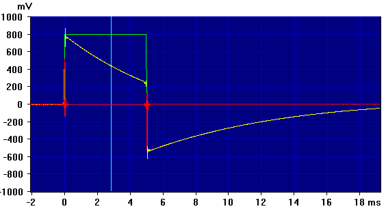
The red trace is the derivative of the input signal, obtained and displayed via:
    Buf0="<=W0"            ;Copy Left In wave to Buf0
    Buf0="<D"              ;Derivative
    Buf0="<dWB0(255,0,0)"  ;Display with solid red line
The derivative is essentially zero everywhere except at the pulse edges, where it shows a 500 mV positive spike on the rising edge and an equal-amplitude negative spike on the falling edge. The amplitudes will be equal regardless of the duration of the original pulse, making falling edge detection much simpler and more reliable.
Total Integration (Summation) and Dot Products:
To find the sum of all elements in Buf0 and assign it to variable X, use X=Buf0?U. This is useful when finding the dot product of two arrays: You first multiply them together, element by element, then find the sum of all the products. For example, the dot product of Buf0 and Buf1 can be found by:
    Buf0="<*B1     ;Multiply Buf0 by Buf1
    X=Buf0?U       ;Sum all Buf0 elements
See the _Phase_Mtr_Task macro in the Phase Meter mini-app for a working example. Note that if the raw data is from an input or output channel, it has a full-scale range of +/-32767. The product of two elements can thus be over a billion, and the sum of all 1024 elements can easily overflow the buffer data format limit of about 2 billion. That's why _Phase_Mtr_Task divides the raw input data by 32767 before finding the dot product.
In addition to the above, the Macro Math Functions topic discusses Sigma (Summation) Functions, BwSig() and BsSig(), which return the effective energy between any two index positions of a given buffer. These operate just like Sigma mode does for the trace cursors.
Peak Functions:
To find the most-positive among all 1024 values in Buf0, use Buf0?p. To find the most-negative, use Buf0?n. After either operation, you can find the index of the peak in read-only variable Posn?p.
Also, Macro Math Functions discusses the pkB(N) and pkb(N) functions, which only find the most-positive peak over either all 1024 or just the first 512 points, respectively. They allow you to specify the buffer number via N, which may be a variable or expression. They also return the index of that peak in read-only variable Posn?p.
You can find the most-extreme (positive or negative) peak by first taking the absolute value with Buf0="<|", then using either Buf0?p or pkB(N).
Index Range Cropping:
Buf0="<o(min,max)" nulls all elements of the Buf0 array except those in (min,max) range, inclusive.
Reversing the order of the index range limits to Buf0="<o(max,min)" nulls all elements within the index range, inclusive.
One use for the first operation is to create a Memory Curve that will correct frequency response over a limited portion of the full spectrum... effectively, a custom Mirror Curve. You might want to do this if you are testing transducers (such as speakers or microphones) whose response falls off and/or is very unpredictable outside the range of interest. If you include those regions in the correction curve, they can result in a distracting display with greatly boosted noise and response irregularities outside the desired region.
See also Macro Overview, Macro Arrays Buf0-Buf7
- Back to Macro Array Copy/Swap Operations
- Ahead to Macro Array Sort Operations
- Daqarta Help Contents
- Daqarta Help Index
- Daqarta Downloads
- Daqarta Home Page
- Purchase Daqarta
Questions? Comments? Contact us!
We respond to ALL inquiries, typically within 24 hrs.INTERSTELLAR RESEARCH:
Over 35 Years of Innovative Instrumentation
© Copyright 2007 - 2023 by Interstellar Research
All rights reserved