Software for Windows
Science with your Sound Card!
Sound Card Multi-Trace Arrays
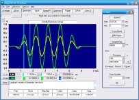
Daqarta trial and Pro-license users can store waveform traces to the Juxt memory array and display them individually or as a multi-trace array. The array traces can be displayed with adjustable spacing for clarity, or superimposed to see small differences.
![[Juxt Array wave traces (47K image)]](JuxtWave.png)
The above example shows the use of frequency modulation (FM) to control waveshape, by setting the modulation frequency to particular ratios of the main tone or "carrier" frequency. This technique is called FM synthesis and was used by early digital music synthesizers because of the wide variety of sound timbres that can be created by varying a few parameters.
These traces were created with the Daqarta Generator using a 440 Hz carrier, with the frequency deviation (depth of modulation) also set to +/-440 Hz. The modulation frequency is shown at the right end of each trace, with 0 at the bottom (no modulation, simple sine wave only), then 110, 220, 440, and 880 Hz.
The 440 Hz trace is highlighted, indicating that it has been selected by clicking on it. All the cursor readouts, Notes, Labels, and Fields, as well as settings in dialogs not shown here, reflect that particular trace.
The Juxt Array dialog at the right shows that Field 4 is used as the label field for each trace. That's the field at the bottom center of the image labeled "FM Mod Freq", with a value of 440. The label field can be set to show any field, or the trace number, or the date or time (if they are not already in fields like they are here).
In this case, the Date and Time field values were entered via CTRL+ALT+D and CTRL+ALT+T, and the other fields were entered manually. But these operations can usually be automated via macro scripts.
The array can be displayed with the traces sorted by the contents of the designated label field and shown in ascending or descending order. (In this example the Sort button was not needed since the traces were acquired in ascending order.) Pressing the "Up" button would change it to "Down", and the same traces would be shown from top to bottom.
The Spacing between the traces was adjusted by holding the ALT key and dragging them apart with the mouse. The entire array can be Offset (shifted higher or lower) by dragging while holding the SHIFT key.
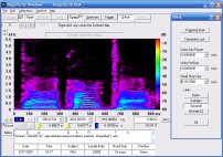
You can superimpose the traces for comparison, by ALT-dragging or setting Spacing to zero. The following example shows the effects of different spectral window functions on a 4000 Hz sine wave:
![[Juxt Array spectra (43K image)]](JxtSpect.png)
Background: The FFT (Fast Fourier Transform) that is used to generate the Spectrum display can only analyze an input signal at discrete frequency steps. These steps are spaced at the sample rate divided by the number of samples analyzed, which here is every 48000 / 1024 = 46.875 Hz.
If the input is a pure sine wave whose frequency falls exactly on one of these steps (which could be achieved by using the Generator in the Step Lines entry mode, for example), the spectrum would consist of nothing but a single vertical line at that frequency. In the more usual case, the signal frequency falls between steps, resulting in spectral leakage to adjacent lines.
In the example the actual input is at 4000 Hz, almost midway between the lines at 3984.375 and 40321.25 Hz. As the trace labeled "None" shows, this is just about the worst possible case for leakage: Even an octave away (2000 Hz, the left margin of this expanded display), the leakage is still nearly one percent (-40 dB).
By applying a window function to the raw data before computing the spectrum, the leakage can be greatly reduced. (See Spectrum Window Theory and Demonstration for a discussion of how this works.) The array shows the result for each of Daqarta's six standard window functions.
Because the array is shown with Spacing set to zero, the traces can be compared directly. You can see that there are trade-offs between initial sharpness and ultimate leakage reduction. For instance, the Hamming trace drops sharply at first, then rebounds such that it is only down -60 dB at the 2 kHz left margin, whereas the Hann trace (highlighted) is not as sharp, but is down more than -100 dB at the margin.
This example also shows trace labels positioned for clarity, instead of all at the right end (default). Each trace was first selected by clicking on it, then its label was dragged while holding down the CTRL key. As you drag horizonally, the label also moves vertically to keep its lower left corner just above the trace.
When an array of traces is saved to a .JXT file, all label positions are saved as well.
Features:
Oscilloscope
Spectrum Analyzer
8-Channel
Signal Generator
(Absolutely FREE!)
Spectrogram
Pitch Tracker
Pitch-to-MIDI
DaqMusiq Generator
(Free Music... Forever!)
Engine Simulator
LCR Meter
Remote Operation
DC Measurements
True RMS Voltmeter
Sound Level Meter
Frequency Counter
Period
Event
Spectral Event
Temperature
Pressure
MHz Frequencies
Data Logger
Waveform Averager
Histogram
Post-Stimulus Time
Histogram (PSTH)
THD Meter
IMD Meter
Precision Phase Meter
Pulse Meter
Macro System
Multi-Trace Arrays
Trigger Controls
Auto-Calibration
Spectral Peak Track
Spectrum Limit Testing
Direct-to-Disk Recording
Accessibility
Data Logger
Waveform Averager
Histogram
Post-Stimulus Time
Histogram (PSTH)
THD Meter
IMD Meter
Precision Phase Meter
Pulse Meter
Macro System
Multi-Trace Arrays
Trigger Controls
Auto-Calibration
Spectral Peak Track
Spectrum Limit Testing
Direct-to-Disk Recording
Accessibility
Applications:
Frequency response
Distortion measurement
Speech and music
Microphone calibration
Loudspeaker test
Auditory phenomena
Musical instrument tuning
Animal sound
Evoked potentials
Rotating machinery
Automotive
Product test
Contact us about
your application!
Questions? Comments? Contact us!
We respond to ALL inquiries, typically within 24 hrs.INTERSTELLAR RESEARCH:
Over 35 Years of Innovative Instrumentation
© Copyright 2007 - 2023 by Interstellar Research
All rights reserved