Gut-Level Fourier Transforms - Part 3:

The Fast Fourier Transform

Previously, we saw how the Discrete Fourier Transform (DFT) computes a spectrum by multiplying the digitized input by sine and cosine waves at each analysis frequency, and summing to find the average value of each frequency component. This involves a lot of (slow) multiplications... over a million for every 1024 input samples.

But it turns out that many of these multiplications are redundant. For example, the sine and cosine waves repeatedly pass through zero, so there is no reason to actually multiply any input sample by zero... we can just omit those calculations.

Similarly, everywhere the sine or cosine wave passes through +1, we can skip the multiply and just add the input sample directly. Where they pass through -1 we just need to subtract instead.

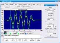
But that's only scratching the surface in the Department of Redundancy Department. Figure 1 shows components of the first four reference frequencies (superimposed), below an arbitrary input waveform:

Fig. 1: Arbitrary Signal and First 4 Reference Components

At each point where two or more components intersect, that single value only needs to be multiplied by the corresponding input value once. Although only sine components are shown here for clarity, cosine components could be superimposed as well to yield additional intersections. It doesn't matter whether an intersection is between sines, cosines, or any combination; each marks a redundant multiplication.

But there are still more redundancies. In places where we would be multiplying an input by a sine or cosine value and by its negative, we can do a single multiply and just negate the result. These places could be visualized as intersections by folding the superimposed sinusoids about the zero line to produce a "full wave rectified" version.

As you can see, there are a fair number of intersections using just the sines of four components; when considering positive and negative versions, and with both sines and cosines of all components (typically 256, 512, or more), the number of redundant points becomes really significant. The difficulty, however, is coming up with a method to keep track of all the values in order to avoid redundant calculations.

One approach, discussed by Chamberlin (see Ref.), is to begin by arranging all the values to be multiplied in a large table of sine and cosine values versus sample numbers. Each row in the table would hold all the values of a single sine or cosine reference; there would be a sine row and a cosine row for each analysis frequency. Each column would thus hold all the values that would need to be multiplied by the corresponding sample number for that column.

The first column of the table, for example, would be all the sine/cosine values that must be multiplied by the first sample... namely, the values associated with an angle of 0. So for each sine frequency row, this entry would be 0, while for each cosine it would be 1.

The places that appeared as intersections of our previous superimposed traces could be noted by scanning down each column and looking for duplicate values. Values that are the same except for a sign change could also be noted. To boil this all down to a general algorithm that eliminated the redundancies, you would need to use trigonometric identities and a LOT of matrix operations... but in principle, it could be done.

However, Cooley and Tukey of Bell Laboratories devised a better way back in the '60s, which became known as the Fast Fourier Transform (FFT). They noted that although the ordinary DFT of N input samples requires N² multiplications, the same set of samples could be separated or "decimated" into two portions (odd and even), each containing N/2 samples. DFTs of those would thus each require only N²/4 multiplications, or a total of N²/2... a savings of half.

The two resulting spectra are not simply halves of the desired total spectrum, but with just a modest additional effort they can be recombined to produce it. If N is a power of two, the decimation process can be repeated until only a bunch of two-sample DFTs remain.

Recall that a DFT of N samples contains N/2 output frequencies, with a sine and cosine version required for each. So with only two samples, we have just one sine and one cosine frequency. But the reference frequencies start at zero phase when multiplying the first input sample, and since the sine of zero is zero and the cosine of zero is one, we don't need any multiplications at all for that sample. So for our two-sample DFTs we only need to perform two multiplications.

Even when we consider the extra multiplications needed to reconstitute the full spectrum from these little "sub-spectra", the net result is that the spectrum can be computed with something like Nlog₂(N) multiplications. For N = 1024, the FFT is thus about 100 times faster than the straightforward DFT.

But the FFT only works if N is a power of 2, whereas the DFT can use any number of samples. For non-real-time analysis, the DFT may still be useful in reducing the "spectral leakage" that results when the transform length is not an integer number of cycles of the waveform being analyzed. We'll cover this in detail next time, then discuss how "windowing" techniques can reduce it.

It turns out that a windowed FFT is usually a better approach than an adjustable DFT length, since you rarely know the exact periodicity of the input signal (relative to the sample rate) ahead of time. Typically, the DFT would only be used to examine an existing set of samples, where you can adjust the DFT length for best results after you preview the data, and where you don't need the speed that the FFT provides for real-time operation.

If you want to experiment with a real-time spectrum analyzer that uses the FFT, you can download the author's Daqarta for Windows software that turns your Windows sound card into a full-fledged spectrum analyzer... and much more.

All Daqarta features are free to use for 30 days or 30 sessions, after which it becomes a freeware signal generator... with full analysis capabilities. (Only the sound card inputs are ignored.)

Reference: Chamberlin, Hal Musical Applications of Microprocessors, Hayden Book Company, 1985. ISBN 0-8104-5768-7