Arbitrary Random Distribution Mini-App

• Introduction
• Operation
• Theory
• Macro Listings:
  • Arb_Rand_Distr
  • _Arb_Distr_Gauss
  • _Arb_Distr_Ctrls
  • _Arb_Distr_CDF
  • _Arb_Distr_Task
  • Arb_iCDF_Test

Introduction:

The Arb_Rand_Distr macro mini-app is included with Daqarta. To run it, first hit CTRL+F8 to open the Macro Dialog. Then scroll the Macro List down and double-click on Arb_Rand_Distr. (There is no single-letter ID for Hot Key access, as there is for the mini-apps at the top of the list.)

Note that you can open this Help topic by clicking anywhere in the Arb_Rand_Distr control dialog.

Arb_Rand_Distr uses the inverse cumulative distribution function (iCDF) to provide a simple way to generate arbitrary non-uniform random distributions. (See Theory below.) By default it creates Gaussian ("normal") distributions with adjustable mean and standard deviation, but you can optionally load any arbitrary shape from a file.

The mini-app plots the target distribution or probability density function (PDF) as well the cumulative distribution function (CDF) and the final iCDF.

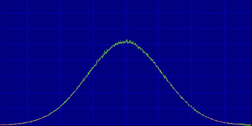
A Histogram button superimposes a scaled copy of the target PDF over the actual histogram of the generated distribution so you can evaluate the fit. As shown here for the default Gaussian distribution, there is a near-perfect match except where the target incidence is very low at the tails; a magnified view would show that the generated version drops off too fast.

You can then save the iCDF array as a file that will allow you to generate the distribution easily from your own macros, using only a single random value per generated sample. You can use the code provided in _Arb_Distr_Task directly, or modify it for your needs.

Operation:

When first started, the Arb_Rand_Distr mini-app sets the Generator to produce a muted uniform white noise. It also calls the _Arb_Distr_Gauss macro to generate a Gaussian ("normal" distribution) curve from the fundamental equation, applying the default Gauss Mean and Gauss Std. Deviation control settings.

Likewise, it calls _Arb_Distr_CDF to generate the special inverse cumulative distribution function (iCDF) array needed to convert uniform random values to the specified distribution. (See Theory, below.)

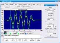
With the Gauss / File button unclicked, toggling the White / Distr button switches to the default Gaussian distribution. The _Arb_Distr_Task macro is installed to generate uniform random values and apply the iCDF to create 1024 Gaussian samples for each trace update. The task is installed such that these samples replace those from the main Generator, so the display shows the waveform of the Gaussian noise instead of the Generator's uniform white noise (which was only for comparison).

Superimposed on the waveform is the Gaussian curve shown in yellow, the CDF shown in red, and the iCDF shown in pink. See Theory, below, for an image and more info.

The Histogram button toggles the main Waveform Averager to begin a histogram of 1024 frames, each of 1024 samples, for a total of 1048576 samples. The display will Pause upon completion. You can toggle Pause off by clicking the button or by hitting ALT+P to resume viewing the raw waveform. Alternatively, you can click Averager (or hit ALT+A) to start another histogram, or do the same thing by toggling the Histogram button off and back on.

If you want to keep the distribution for use in your own macros (or even for use with other software), click the Save iCDF File button. You will be prompted to save a .BUF file, which is a direct copy of the iCDF for use in Daqarta (1024 values, each consisting of a 32-bit integer and a 32-bit fraction). You can instead choose to save a .TXT file via the file type selector drop-down control at the bottom of the dialog. This will also work fine with Daqarta (although slightly larger and slightly slower to load), and will be compatible with other software as well as viewable in any text editor.

Avoid .DQA, .WAV, or .DAT formats. These are intended for raw waveform data and are limited to 16-bit integers. Since the iCDF consists of real values between 0 and 1024, you would get only 10-bit resolution. That results in a noticeably inferior histogram, with conspicuous steps and jagged spikes.

There are numerous published methods to create Gaussian random values from uniform random numbers, and they have various virtues and shortcomings. The main utility of the Arb_Rand_Distr mini-app is that you can create virtually any distribution, and do it with only a single uniform random value per sample.

To demonstrate, toggle Histogram and White / Distr off and click the Gauss / File button on. Select the Cos2HiLo.TXT file, then toggle White / Distr back on. This file consists of 2 "raised inverted cosine" cycles, with the second cycle half the amplitude of the first. The histogram thus begins at zero for max negative values, rises to a peak at -50% negative values, falls to zero at the center for values of 0, rises to a half-sized peak at +50% positive values, and back to zero for max positive values.

The only requirement of the file is that it have 1024 points. Text (.TXT) files are usually convenient, especially if they are created by other software. You can also use the Daqarta Generator to create .DQA, .WAV, or .DAT files for this purpose. Unlike saving the iCDF, these formats are fine for the raw distribution as long as you use the full 16-bit range (typically, Stream Levels total 100%).

Note: As mentioned in the Introduction, the iCDF method produces a histogram that drops off too abruptly at near-zero incidence regions, like the tails of a Gaussian or the central null of the Cos2HiLo distribution.

But there is also a further artifact you might encounter with very low Gauss Std. Deviation settings and similar narrow custom distributions: The positive tail may drop off slightly sooner than the negative. This is not easy to see on the histogram, but can be very obvious on the raw noise waveform. The narrow deviation means the noise waveform is mostly near zero, except for occasional spikes due to the tails of the distribution. Due to the assymetry, there may be conspicuously more negative spikes than positive spikes.

Theory:

The basic idea of this mini-app is to generate an ordinary uniform random real number in the range of 0-1024, then convert it into the desired distribution by means of interpolation from a lookup table of 1024 values. This is followed by possible scaling and/or offset to fit a desired range.

The trick is to create the proper table. We start with the desired distribution, which is known as the probability density function (PDF). We use an array of 1024 values in Buf0 for the PDF, either obtained by computation of a Gaussian curve, or by loading from a file. In the following discussion we will use the default Gaussian distribution, shown in yellow below:

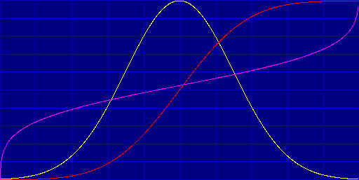
The PDF is essentially a graph of the height of the desired histogram for each output value, from the most negative to the most positive. The yellow curve indicates that the histogram should have very few extreme values (the tails), while it should have many values near the mean of zero (the central peak).

Since we will be using input values in the range of 0-1024, and since we will have only 1024 values in the final lookup table, it follows that most of those table values must also cluster around the mean, with relatively fewer for the tails. In other words, at the center of the table the values will change very little from one position to the next, while at the ends the change will be much greater.

The first step in creating this table is to create an intermediate array called the cumulative distribution function (CDF), shown in red above and stored in Buf1. This is a integration of the PDF: we step through the PDF from left to right (negative to positive), adding each PDF value to a running total which also becomes the current CDF value. The CDF thus grows from zero at the start to 100% at the end.

The PDF is thus the slope of the CDF. Note that the CDF starts out very flat (low slope) where the negative tail of the PDF is very small. It gently becomes steeper until it is steepest at the center (the peak of the PDF), then slowly flattens out as it continues to rise, becoming very flat once again as it nears 100%, where the positive tail of the PDF is again very small.

Notice that the CDF is the opposite of what we want: It changes slowly at the ends and rapidly in the center, whereas we want our final table to change rapidly at the ends and slowly in the center. So we need to "invert" the CDF to create the inverse CDF (iCDF) shown in pink.

This is essentially the same as drawing 1024 horizontal lines across the CDF, with equal vertical spacing, and reading the corresponding X value where each horizontal line intersects the CDF. In the _Arb_Distr_CDF macro this is done by scanning CDF values in Buf1 until just past each integer Y value, then interpolating to find the corresponding X. That X value is then stored in the iCDF output table Buf2 at the index corresponding to the integer Y of the CDF. The result is a table of 1024 output (Y) values corresponding to each input (X) value from the uniform 0-1024 random source, used by the _Arb_Distr_Task macro to create the desired distribution.

Arb_Rand_Distr Macro Listing:

    ;<Help=H490A
    Sgram=0
    Spect=0
    A.LoadGEN="WhiteMute"
    Gen=1
    Xpand=0
    VolMastL=-200
    E.IF.VolWaveL=
        VolWaveL=-200
    ENDIF.
    WavgMode=Hist
    WavgFrames=1024

    Ctrls="<<Arbitrary Random Distribution"

    Ctrl0="<< Gauss Mean"
    Ctrl0="<S(-0.5, 0.5)"
    Ctrl0="<u"
    Ctrl0=0

    Ctrl1="<<Gauss Std. Deviation"
    Ctrl1="<S(0.1,5.0)"
    Ctrl1="<u"
    Ctrl1=1.0

    Ctrl2="<X"
    Ctrl3="<X"

    Btn0="Gauss / File"
    Btn0="<T"
    Btn0=0

    Btn1="White / Distr"
    Btn1="<T"
    Btn1=0

    Btn2="Histogram"
    Btn2="<T"
    Btn2=0

    Btn3="Save iCDF File"
    Btn3="<M"
    Btn3="<D"

    @_Arb_Distr_Gauss
    @_Arb_Distr_CDF
    @_Arb_Distr_Ctrls=Ctrls
    Task="-_Arb_Distr_Task"
    Buf0="<d-"
    Buf1="<d-"
    Buf3="<d-"
    Buf5="<d-"
    Avg=0
    A.LoadGEN="Setup"
    

_Arb_Distr_Gauss Macro Listing:

    ;<Help=H490A
    UX=0
    M=Ctrl0
    D=Ctrl1 * 0.15
    C=sqrt(2 * pi)
    WHILE.UX=<1024
        X=(UX-511.5)/1024
        Z=(X-M)/D
        Buf0[UX]=exp(-Z^2 / 2) / C
        UX=UX+1
    WEND.
    

_Arb_Distr_Ctrls Macro Listing:

    ;<Help=H490A
    IF.Ctrls=0                 ;Mean
        @_Arb_Distr_Gauss      ;Recompute Gaussian
        @_Arb_Distr_CDF        ;Recompute CDF, iCDF
    ENDIF.

    IF.Ctrls=1                 ;Std Deviation
        @_Arb_Distr_Gauss      ;Re-compute Gaussian
        @_Arb_Distr_CDF        ;Recompute CDF, iCDF
    ENDIF.

    IF.Ctrls=4                 ;Gauss/File button
        IF.Btn0=1              ;If File,
            Buf0="<LoadTXT:"   ; load it now
            IF.Buf0?L=0        ;If file not loaded,
                Btn0=0         ; button up for Gauss
            ELSE.              ;If file loaded,
                N=Buf0?n       ; find most-neg value
                IF.N=<0        ;If actually negative,
                    Buf0="<-(N)"   ;Shift up to zero
                ENDIF.
                Ctrl0="<D"     ;Disable Mean for File
                Ctrl1="<D"     ;Disable Std Dev for File
                @_Arb_Distr_CDF  ;Compute CDF, iCDF for File
            ENDIF.
        ELSE.                  ;If Gauss,
            Ctrl0="<N"         ;Enable Mean
            Ctrl1="<N"         ;Enable Std Dev
            @_Arb_Distr_Gauss  ;Recompute Gaussian
            @_Arb_Distr_CDF    ;Recompute CDF, iCDF
        ENDIF.
    ENDIF.

    IF.Ctrls=5                 ;White/Distr button
        IF.Btn1=1              ;If Distr,
            Btn0="<D"          ;Disable Gauss/File button
            Btn3="<N"          ;Enable Save iCDF button
            Task="*_Arb_Distr_Task"     ;Install Task
            Buf0="<dWU"        ;Show PDF
            Buf1="<dWU"        ;Show CDF
            Buf3="<dWU"        ;Show iCDF
            IF.Btn2=1                      ;If Hist on,
                Buf5="<dWU(255,128,128)"   ;Show scaled PDF
            ENDIF.
        ELSE.                  ;If White,
            Btn0="<N"              ;Enable Gauss/Dist
            Btn3="<D"              ;Disable Save
            Task="-_Arb_Distr_Task" ;Uninstall Task
            Buf0="<d-"             ;No PDF display
            Buf1="<d-"             ;No CDF display
            Buf3="<d-"             ;No iCDF display
            Buf5="<d-"             ;No scaled PDF for Hist
        ENDIF.
    ENDIF.

    IF.Ctrls=6                 ;Histogram button
        IF.Btn2=1              ;If on,
            Avg=1              ;Start Hist Avg
            IF.Btn1=1          ;If Distr,
                Buf5="<dWU(255,128,128)"   ;Show scaled PDF
            ENDIF.
            Buf0="<d-"         ;No PDF display
            Buf1="<d-"         ;No CDF display
            Buf3="<d-"         ;No iCDF display
        ELSE.                  ;If Hist off,
            Avg=0              ;Histogram off
            Pause=0            ;UnPause if needed
            IF.Btn1=1          ;If Distr,
                Buf0="<dWU"    ;Show PDF
                Buf1="<dWU"    ;Show CDF
                Buf3="<dWU"    ;Show iCDF
            ENDIF.
        ENDIF.
    ENDIF.

    IF.Ctrls=7                 ;Save iCDF File button
        Buf2="<Save:"              ;Open Save dialog
        IF.Buf2?S=0                ;If no data saved,
            Msg="File not Saved"   ;Show message
        ELSE.
            Msg="File saved OK"
        ENDIF.
    ENDIF.

_Arb_Distr_CDF Macro Listing:

    ;<Help=H490A
    ;Compute CDF in Buf1 from PDF in Buf0:
    UI=0                           ;Initialize index
    S=0                            ;Initialize sum
    WHILE.UI=<1024                 ;Do 0-1023
        S=S+Buf0[UI]               ;Add PDF value to sum
        Buf1[UI]=S                 ;Sum to CDF
        UI=UI+1                    ;Next index
    WEND.

    ;Compute iCDF from CDF:
    Buf1="<*(1024/Buf1[1023])"     ;Normalize CDF to 1024 max
    Buf2[0]=0                      ;iCDF starts at 0
    UY=1                           ;Start scan at index 1
    UX=1
    WHILE.UY=<1024                 ;Do 1-1023
        WHILE.UX=<1024
            B=Buf1[UX]             ;Get CDF value
            IF.B=>=UY              ;At/past current Y step?
                A=Buf1[UX-1]       ;If so, get prior CDF for interp
                Buf2[UY]=(UY-A) / (B-A) + UX - 1   ;Interp for iCDF
                UY=UY+1            ;Next Y step
                LoopBreak=2        ;Exit this WHILE loop
            ELSE.                  ;Else if below current Y step,
                UX=UX+1            ;Try next X value
            ENDIF.
        WEND.
    WEND.

    ;Create scaled 512-point PDF in Buf5 for Hist display:
    Buf5="<=(0)"                   ;Clear Buf5
    UX=0
    WHILE.UX=<512                  ;Do 0-511
        Buf5[UX]=(Buf0[2*UX] + Buf0[2*UX+1])/2 ;Avg 2 PDF points
        UX=UX+1                    ;Next Hist point
    WEND.
    Buf5="<*(255*512/S)"           ;Scale Buf5 for Hist display

    ;Scale PDF, CDF, and iCDF for display:
    Buf0="<*(65535 / pkB(0))"      ;Normalize PDF to peak
    Buf1="<*(65535 / Buf1[1023])"  ;Normalize CDF to final sum
    Buf3="<=B2"                    ;Copy of iCDF for display
    Buf3="<*(65535/Buf3[1023])"    ;Normalize iCDF to max value

_Arb_Distr_Task Macro Listing:

    ;<Help=H490A
    UJ=0
    WHILE.UJ=<1024                 ;Do UJ = 0-1023
        R=rnd(0,1024)              ;Uniform random value 0-1024
        Buf4[UJ]=64 * (Buf2?i[R] - 512)    ;Interp iCDF to Buf4
        UJ=UJ+1                    ;Next index
    WEND.
    Buf4="<uW2"                    ;Upload Buf4 as raw Left Out data

Arb_iCDF_Test Macro Listing:

This is not part of the Arb_Rand_Distr mini-app. It is a separate macro to allow you to test iCDF files created by Arb_Rand_Distr. It uses the same _Arb_Distr_Task macro from Arb_Rand_Distr.

When you invoke this macro it first tests to see if _Arb_Distr_Task is already installed. If so, it just uninstalls it and exits. Otherwise, it prompts you to load a file. If it loads OK, the macro installs _Arb_Distr_Task as a {\i pre-process} task, which means that it runs before normal main Daqarta raw data processing. That way, when _Arb_Distr_Task uploads a new set of 1024 samples before each trace update, it will be treated like ordinary data... you can take the Histogram, Spectrum, or whatever you want.

When you are done testing the iCDF, run this macro again to uninstall _Arb_Distr_Task.

    ;<Help=H490A
    Task="?_Arb_Distr_Task"
    IF.Task=1
        Task="-_Arb_Distr_Task"
    ELSE.
        Buf2="<Load:"
        IF.Buf2?L=>0
            Task="*_Arb_Distr_Task"
        ENDIF.
    ENDIF.