Sound Card FFT Filter Mini-App

• Introduction
• FFT_Filter Macro Listing
• _Filt_Limits Macro Listing
• _Filt_Ctrls Macro Listing
• _Filt_Task Macro Listing

Introduction:

The FFT_Filter macro mini-app is included with Daqarta. To run it, hit the F8 key followed by the SHIFT+F keys. Note that this macro ID is case-sensitive because the Missing Fundamental macro uses a lowercase f as its ID.

Alternatively, hit CTRL+F8 to open the Macro Dialog and double-click on FFT_Filter in the Macro List.

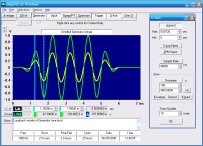
FFT_Filter demonstrates the use of the FFT (Fast Fourier Transform) and IFFT (Inverse Fast Fourier Transform) to create a "brick wall" filter and apply it to various signals. The filtered signal is shown on the same trace as the raw signal, in waveform or spectrum display mode.

FFT_Filter uses a Custom Controls dialog to allow adjustment of various parameters. You can adjust the lower and upper frequency limits of the filter, as well as the frequency and waveform of a test signal from the Daqarta Generator. A button changes the channel to be filtered, allowing input signals instead of the default Generator signal.

In addition there are controls to adjust the vertical position of the filtered signal, its line style, and its color.

Note that you can open this Help topic by clicking anywhere in the FFT_Filter control dialog.

The default test waveform is a square wave at 1000 Hz, with the default filter passing 0-6000 Hz. In waveform display mode, a separate dashed red line at the top of the screen shows the shape of the filter as if it were a spectrum display. Since Spectrum mode extends from 0-24000 Hz (assuming the default 48000 Hz sample rate), the red line is high for the first quarter (6000 / 24000) of the uneXpanded waveform display, and low for the rest.

However, eXpand (the X-Axis button) is active by default and set to show only the first 2 msec of the waveform, for ease of viewing the effects of the filter on the square wave. The red line is thus high all the way across the display. Just toggle the X-Axis button off to see the full shape.

(In Spectrum display mode the red line is not shown, since the filtered region is usually obvious.)

Since a square wave contains a series of odd harmonics, the filter passes 1000, 3000, and 5000 Hz only, which are visible as ripples on the basic square waveform display. If you reduce the upper limit to (say) 2000 Hz, only the 1000 Hz fundamental sine wave remains. If you set the lower limit to 2500 and the upper to 3500, you get only the 3000 Hz third harmonic.

If you set the lower limit to a higher frequency than the upper limit, the filter becomes a "gap" filter that removes only the frequencies between the limits. So if you set the lower limit to 3500 and the upper to 2500, only the 3000 Hz third harmonic of the square wave is removed.

To apply the filter to file data, you must start FFT_Filter first. That starts the Generator by default, which disables the DD/Open button, so you must manually toggle Generator off in order to open the desired file.

Long (DDisk) files can be viewed "live" by hitting unPause. With Trigger active the original data and the filter output will appear much like it would have when originally recorded. However, you may want to get a "slow motion" view by setting a low Read Step Size in the DDisk Controls dialog, then toggling Trigger off to get a slow-scrolling free-run display.

Static files (1024 samples, filling only a single screen) can also be filtered. This is the same as the Paused view of a live trace. (You may actually prefer to Pause a live trace to see the effects of the filter limits, since the controls are much more responsive. See the _Filt_Ctrls discussion below.)

FFT_Filter works fairly well to display a filtered version of an arbitrary file, such as to remove noise or interference. But note that it only shows one screen at a time, just as if you were viewing it live. You might think that you could use this filter pretty much as-is to convert an entire long file, by applying it to each 1024-sample segment in turn, and splicing the filtered results together. But there is a problem with that.

To see the problem, start FFT_Filter and observe the default 1000 Hz square wave. Now open the Trigger control dialog and slowly increment Delay. You'll see the overall square wave move to the left, but pay attention to the filtered response of the first high phase. You'll see that as this initial square phase becomes smaller (because the trigger point is effectively off-screen to the left), the response starts to change. When the first high phase is about half the original width, the response is drastically different... even though the response in subsequent cycles is fairly constant.

This shows that the filter has problems at the start of the 1024-sample section it is working on, and it has the same problem at the end as well. If you attempt to apply it to an arbitrary file in 1024-sample sections, there will be artifacts at each splice.

One way to deal with this is to use a "windowed overlap and add" scheme. You filter one 1024-sample section, then apply a window function to it, similar to the window functions used to reduce spectral leakage. This preserves the middle part and tapers to nothing at either end. Then you advance only 512 samples and repeat. This second section is now added to the first such that the original sample numbers align. This adds the tapered-out start of the second section to the unaffected middle of the first, and the middle of the second to the tapered-out end of the first. The window function is chosen such that the taper-down of the first exactly balances the taper-up of the second, so that by repeating this process the entire file is filtered.

FFT_Filter invokes macros called _Filt_Limits, _Filt_Ctrls, and _Filt_Task. Each is discussed individually below, with listings.

FFT_Filter Macro Listing:

The FFT_Filter macro sets Trigger on and sets waveform display mode by forcing Spectrum and Spectrogram (Sgram) modes off. It sets the Spectrum Window type to Hann but toggles it off, to be used for later experiments (see below). It sets the waveform eXpand limits to show only the first 2 msec of the filtered waveform, then toggles eXpand on.

After loading the FFT_Filter.GEN setup for the default Generator square wave, FFT_Filter prepares the Custom Controls dialog by setting control labels, types, ranges, and initial values.

After setting the initial values of the lower (Ctrl0) and upper (Ctrl1) limit frequencies, it calls the _Filt_Limits macro to translate those values into the filter shape in Macro Array Buf0. (_Filt_Limits is also called by _Filt_Ctrls when either of the limits is changed.)

FFT_Filter then sets working variables for the channel (UC), waveform (UW), line style (US), and color (UH).

It also sets the zero positions and line styles of Buf1 and Buf2, which will be displayed as the filtered trace and the dashed red filter limits trace, respectively. For Buf2, the display mode (Waveform Bipolar) and red color (255,0,0) are set along with the dashed line style (1) by a single Buf2="<dWB1(255,0,0)" command.

FFT_Filter next installs a multitasking macro called _Filt_Task that does the actual filtering and display. Finally, it launches the Custom Controls dialog handler called _Filt_Ctrls, which behaves as a loop of indefinite duration.

FFT_Filter then waits until the dialog is eventually closed (ending the "loop"), after which it uninstalls _Filt_Task and clears the Buf1 and Buf2 traces from the screen.

;<Help=H4906
Close=
Trig=1
TrigLevel=0
TrigDelay=0
Spect=0
SpectWind=Hann
SpectWindOn=0
Sgram=0
XpandMin=0
XpandMax=2m
Xpand=1

A.LoadGEN="FFT_Filter"
Ctrls="<<FFT Filter"

Ctrl0="<<Lower Limit Frequency"
Ctrl0="<S(0,24k)"
Ctrl0=0

Ctrl1="<<Upper Limit Frequency"
Ctrl1="<S(0,24k)"
Ctrl1=6000
@_Filt_Limits

Ctrl2="<<Left Out Frequency"
Ctrl2="<S(100,24k)"
Ctrl2=1000

Ctrl3="<<Filtered Response Posn"
Ctrl3="<S(-128,128)"
Ctrl3=0
Buf1#Z=Ctrl3

UC=2
Btn0="Filter = " + UC(c)
Btn0="<M"

UW=3
Btn1="Square"
Btn1="<M"

US=2
Btn2="Dotted Line"
Btn2="<M"
Buf1#Y=US

UH=1
H=255
Btn3="Yellow"
Btn3="<M"

Buf2="<dWB1(255,0,0)"
Buf2#Z=64
Task="_Filt_Task"
@_Filt_Ctrls=Ctrls
Task="-_Filt_Task"
Buf1="<d-"
Buf2="<d-"

_Filt_Limits Macro Listing:

This macro is called initially by FFT_Filter, and subsequently by _Filt_Ctrls whenever the lower (Ctrl0) or upper (Ctrl1) filter limits (cutoffs) are changed. It uses these values to compute the filter array in Buf0 that will subsequently be used by _Filt_Task to do the actual filtering.

The array is simply the shape of the desired filter spectrum. Since this is a "brick wall" filter, it consist of ones at all frequencies to be passed, and zeros at all frequencies to be blocked. The array is considered to be 512 pairs of complex (real and imaginary) data points, one pair for each of the possible spectral lines.

_Filt_Limits then copies Buf0 to Buf2 and multiplies that by 16384 to be used as the dashed red filter limits trace in waveform mode. Buf2 will be shown as 1024 wavform points, not 512 complex spectrum points, but this works out because the points are either two zeros or two ones in succession.

_Filt_Limits is intended to be as simple as possible, and in FFT_Filter it makes a dramatic demonstration of the general method, but it's not an ideal filter for every purpose. The problem is that an abrupt cutoff in the frequency domain results in an extended response in the time domain... low-level "ringing" at the cutoff frequency, caused by Gibbs phenomenon.

This is most-easily visible using the Sine waveform. In Spectrum display mode with Spectrum Window off (default), note the location of the high-frequency cutoff. (The same effect applies to the low cutoff as well.) You'll notice that at most signal frequencies you try there are substantial spectral leakage "skirts" draping down from the signal peak, and the cutoff just slices off the skirt above that limit.

Then toggle the Window on using ALT+W (or open the Spectrum controls dialog and click Window). You will see the skirts drop away dramatically, exposing a very thin peak (single spectral line) at the cutoff frequency. It is always lower in amplitude than the skirt was at that point, and typically too small to be seen in a waveform display, but it is actually present nevertheless. If this filter was intended to process audio signals, the ringing could be audible.

To reduce the ringing, it is necessary to reduce the abruptness of the cutoff transition. The simplest way to do this is to apply a smooth cosine-type curve to the transition, as in the Burst Shape applied to the Rise and Fall phases of the Tone Burst function of the Generator.

You could modify _Filt_Limits to compute this by using the cos() math function, which would make it much more involved. Alternatively, you could create a file holding the desired filter shape and load it directly into the Buf0 array, eliminating _Filt_Limits completely. Just remember that the file must consist of 512 pairs, one pair per spectral line, and the values in each pair should be equal.

Actually, there is no reason that the filter needs to be limited to a single passband, or even contain discrete bands. Your filter can be any shape you can compute or otherwise obtain, such as the inverse of a microphone or speaker response curve.

;<Help=H4906
L=Ctrl0 * 1024 / SmplRate
U=Ctrl1 * 1024 / SmplRate
IF.L=>U
    A=L
    L=U
    U=A
    A=1
    B=0
ELSE.
    A=0
    B=1
ENDIF.
I=0
WHILE.I=< L
    Buf0[2*I]=A
    Buf0[2*I+1]=A
    I=I+1
WEND.
WHILE.I=<U
    Buf0[2*I]=B
    Buf0[2*I+1]=B
    I=I+1
WEND.
WHILE.I=< 512
  Buf0[2*I]=A
  Buf0[2*I+1]=A
  I=I+1
WEND.

Buf2="<=B0"
Buf2="<*(16384)"

_Filt_Ctrls Macro Listing:

This macro is invoked by FFT_Filter via @_Filt_Ctrls=Ctrls. This has the general form of an invoked macro loop, with Ctrls as the loop count. In reality, this statement opens a Custom Controls Dialog and waits for a control change, whereupon it calls _Filt_Ctrls and then goes back to waiting for the next control change. The "wait loop" doesn't exit and return to FFT_Filter until the dialog is closed by clicking the "OK" button or the [x] in the title bar.

When a control is changed, _Filt_Ctrls is called with an event code in the Ctrls variable that identifies the control. The changed value itself is in the relevant Ctrl0 to Ctrl3 variable, or the state of Btn0 to Btn3 for toggle-type buttons.

Ctrl0 (code 0) and Ctrl1 (code 1) are the lower and upper filter limits, so these call _Filt_Limits to update the Buf0 filter array.

Ctrl2 (code 2) is Left Out Frequency and Ctrl3 (code 3) is Filtered Response Posn.

Btn0 (code 4) is the Filter channel selector. This button was set by FFT_Filter as a momentary (non-toggle) type via Btn0="<M", so Btn0 doesn't hold a state (as it would in a toggle type). Instead, FFT_Filter set variable UC to 2 to specify Left Out. When Btn0 is pressed, the IF.Ctrls=4 section adds 1 to UC and then ANDs the result with 3 via UC=(UC+1) & 3. This cycles UC from 2 to 3, then to 0, 1, 2 and so on. The button label is updated to show the current channel via the string expression Btn0="Filter = " + UC(c), which uses the (c) Channel Name Format to show variable UC.

Btn1 (code 5) is the waveform selector. It uses variable UW, which was pre-set by FFT_Filter to Wave number 3 for Square. Succesive clicks increment Btn1 until it hits 10 (Noise Band), after which is rolls back to 0 (Sine). However, there is a possible problem at 5 (Arb) and 6 (Play), since these expect user-specified files that are not loaded by the default FFT_Filter.GEN setup. If an attempt to set Left Out Wave to either of these does not return the expected value, the UW variable is incremented to try the next wave type.

Btn2 (code 6) selects the line style, using variable US and cycling it from the default of 2 (Dotted) through 4 (Dash-Dot_Dot) and back to 0 (Solid). The actual style is set via Buf1#Y=US.

Btn3 (code 7) selects the filtered trace color, cycling variable UH through 0-7 using UH=(UH+1) & 7. The actual color setting is done from variable H, which is obtained via H=256 * UH - 1 to conform to the linear hue scheme used by the colr() function. Here H moves only among the major hues (Red, Yellow, Green, etc) except for the special case where UH = 6, when H=1663 is substituted to get middle gray. The actual color is set from H in _Filt_Task using Buf1="<dSU(colr(H))" for Spectrum display mode or Buf1="<dWB(colr(H))" for waveform more.

Control changes can only affect the visible display when it is updated. This happens regularly when the trace is "live", but not when it is Paused (which is the default state for file data). To insure that controls promptly affect the display, TraceUpdate#!=1 forces an update if Pause is active. Note that this happens regardless of which Ctrls event code is received. With a Paused trace, filter limit controls are much more responsive since there is no waiting for a waveform trigger event to update the display.

;<Help=H4906
IF.Ctrls=0
    @_Filt_Limits
ENDIF.

IF.Ctrls=1
    @_Filt_Limits
ENDIF.

IF.Ctrls=2
    L.0.ToneFreq=Ctrl2
ENDIF.

IF.Ctrls=3
    Buf1#Z=Ctrl3
ENDIF.

IF.Ctrls=4
    UC=(UC+1) & 3
    Btn0="Filter = " + UC(c)
ENDIF.

IF.Ctrls=5
    UW=UW+1
    IF.UW=>10
        UW=0
    ENDIF.
    IF.UW=0
        Btn1="Sine"
    ENDIF.
    IF.UW=1
        Btn1="Triangle"
    ENDIF.
    IF.UW=2
        Btn1="Ramp"
    ENDIF.
    IF.UW=3
        Btn1="Square"
    ENDIF.
    IF.UW=4
        Btn1="Pulse"
    ENDIF.
    IF.UW=5
        L.0.Wave=UW
        IF.L.0.Wave=!5
            UW=UW+1
        ELSE.
            Btn1="Arb"
        ENDIF.
    ENDIF.
    IF.UW=6
        L.0.Wave=UW
        IF.L.0.Wave=!6
            UW=UW+1
        ELSE.
            Btn1="Play"
        ENDIF.
    ENDIF.
    IF.UW=7
        Btn1="White Noise"
    ENDIF.
    IF.UW=8
        Btn1="Gauss Noise"
    ENDIF.
    IF.UW=9
        Btn1="Pink Noise"
    ENDIF.
    IF.UW=10
        Btn1="Noise Band"
    ENDIF.
    L.0.Wave=UW
ENDIF.

IF.Ctrls=6
    US=US + 1
    IF.US=>4
        US=0
    ENDIF.
    IF.US=0
        Btn2="Solid Line"
    ENDIF.
    IF.US=1
        Btn2="Dashed Line"
    ENDIF.
    IF.US=2
        Btn2="Dotted Line"
    ENDIF.
    IF.US=3
        Btn2="Dash-Dot Line"
    ENDIF.
    IF.US=4
        Btn2="Dash-Dot-Dot Line"
    ENDIF.
    Buf1#Y=US
ENDIF.

IF.Ctrls=7
    UH=(UH+1) & 7
    IF.UH=0
        Btn3="Red"
    ENDIF.
    IF.UH=1
        Btn3="Yellow"
    ENDIF.
    IF.UH=2
        Btn3="Green"
    ENDIF.
    IF.UH=3
        Btn3="Cyan"
    ENDIF.
    IF.UH=4
        Btn3="Blue"
    ENDIF.
    IF.UH=5
        Btn3="Magenta"
    ENDIF.
    IF.UH=6
        Btn3="Gray"
    ENDIF.
    IF.UH=7
        Btn3="White"
    ENDIF.
    H=256 * UH - 1
    IF.UH=6
        H=1663
    ENDIF.
ENDIF.

IF.Pause=1
    TraceUpdate#!=1
ENDIF.

_Filt_Task Macro Listing:

The filter works by taking the Fast Fourier Transform (FFT) of the raw signal to get the raw (complex) spectrum, just as in Spectrum display mode. (The Spectrum mode goes one step farther and computes the magnitude spectrum for display.) An Inverse FFT (IFFT) can extract the original waveform from the complex spectrum... the process is completely reversible.

The filter action arises by removing unwanted components (spectral lines) from the complex spectrum, before the IFFT converts it back to a waveform... which then lacks those components.

The _Filt_Limits macro computed an array (Buf0) that has 1s at all the spectral lines we want to keep, and 0s at all the unwanted lines. The idea is that if we multiply an array holding the FFT of the signal by this Buf0 array, then at every line where there is a 1 in Buf0, the spectrum is unaffected. Everywhere there is a 0, that line of the spectrum is completely removed.

_Filt_Task thus captures the raw signal waveform to Buf1 via Buf1="<=W(UC)", then scales the raw 16-bit sound card data to better fit the 32-bit FFT using Buf1="<*(32768)". (See the scaling discussion under Inverse FFT Operations in the Macro Array Spectrum (FFT) Operations topic.)

_Filt_Task converts Buf1 to a complex spectrum via Buf1="<fB1", then multiplies each line of the spectrum by the corresponding line in the Buf0 filter array with Buf1="<*B0". Finally, it takes the inverse FFT with Buf1="<iB1" to get the filtered waveform into Buf1.

The remainder of _Filt_Task has to do with displaying the result. If Spectrum mode is active the Buf1 display mode is set accordingly to Spectrum Unipolar, with the color set from variable H selected by Btn3 in _Filt_Ctrls. Then Buf1 is scaled up by 2048, and if a Spectrum Window is active a windowed spectrum is obtained via Buf1="<FB1", otherwise an unwindowed spectrum via Buf1="<fB1". After additional scaling by 2, the magnitude spectrum is found via Buf1="<mB1".

If Spectrum mode is not active, waveform display mode is assumed. The Buf1 display mode is set to Waveform Bipolar with the chosen color via Buf1="<dWB(colr(H))", then the data is scaled down via Buf1="</(16)".

;<Help=H4906
Buf1="<=W(UC)"
Buf1="<*(32768)"
Buf1="<fB1"
Buf1="<*B0"
Buf1="<iB1"

IF.Spect=1
    Buf1="<dSU(colr(H))"
    Buf1="<*(2048)"
    IF.SpectWindOn=1
        Buf1="<FB1"
    ELSE.
        Buf1="<fB1"
    ENDIF.
    Buf1="<*(2)"
    Buf1="<mB1"
ELSE.
    Buf1="<dWB(colr(H))"
    Buf1="</(16)"
ENDIF.

See also Macro Examples and Mini-Apps