Software for Windows
Science with your Sound Card!
Features:
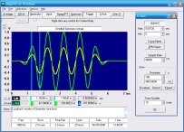
Oscilloscope
Spectrum Analyzer
8-Channel
Signal Generator
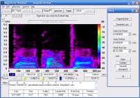
Spectrogram
Pitch Tracker
Pitch-to-MIDI
DaqMusiq Generator
(Free Music... Forever!)
Engine Simulator
LCR Meter
Remote Operation
DC Measurements
True RMS Voltmeter
Sound Level Meter
Frequency Counter
Period
Event
Spectral Event
Temperature
Pressure
MHz Frequencies
Data Logger
Waveform Averager
Histogram
Post-Stimulus Time
Histogram (PSTH)
THD Meter
IMD Meter
Precision Phase Meter
Pulse Meter
Macro System
Multi-Trace Arrays
Trigger Controls
Auto-Calibration
Spectral Peak Track
Spectrum Limit Testing
Direct-to-Disk Recording
Accessibility
Data Logger
Waveform Averager
Histogram
Post-Stimulus Time
Histogram (PSTH)
THD Meter
IMD Meter
Precision Phase Meter
Pulse Meter
Macro System
Multi-Trace Arrays
Trigger Controls
Auto-Calibration
Spectral Peak Track
Spectrum Limit Testing
Direct-to-Disk Recording
Accessibility
Applications:
Frequency response
Distortion measurement
Speech and music
Microphone calibration
Loudspeaker test
Auditory phenomena
Musical instrument tuning
Animal sound
Evoked potentials
Rotating machinery
Automotive
Product test
Contact us about
your application!
Multiple Meters/Plotter/Logger Mini-App
- Introduction
- Quick Start
- Control Operation
- Plotter
- Data Logging
- Measurement Modes
- RMS
- RMS - All Samples
- RMS - Main Trig Sync
- RMS - Chan Sync
- Untriggered RMS - All Samples
- Peak Modes (Pk-Pk, Pos, Neg, Abs)
- dB Re: 1V Sine (dBV)
- dB Re: FS Sine (dBFS)
- Crest Factor and Crest dB
- Frequency
- RMS
- Meter Time Constant
- Macro Array Memory Usage
- Multi_Meters Macro Listing
- Changing Meter Colors
- _Multi_Mtr_Ctrls Macro Listing
- _Multi_Mtr_Mode Macro Listing
- _Multi_Mtr_Task Macro Listing
- _Multi_Mtr_Update Macro Listing
Introduction:
The Multi_Meters macro mini-app included with Daqarta allows simultaneous independent voltage and/or frequency measurement on all active stereo channels (including Multi-Channel Outputs that are set to be monitored as the normal stereo Left Out and/or Right Out.) It shows a separate Custom Meter for each channel, displaying one of 10 measurement types selected for that channel. Alternatively, each meter can show all 10 measurements for the channel.
The measurements for each channel are:
- RMS, mV (3 mode options)
- Peak-to-Peak, mV
- Positive Peak, mV
- Negative Peak, mV
- Absolute Peak, mV
- dB Re: 1V Sine (dBV)
- dB Re: FS Sine (dBFS)
- Crest Factor (Peak / RMS)
- Crest dB (Crest Factor, in dB)
- Frequency, Hz
Note: Voltage measurements will only be correct if you have performed a complete calibration, including at least Auto-Calibration and Full-Scale Range. dB Re: FS Sine requires at least Auto-Calibration. The two Crest modes and Frequency do not require any calibration.
Multi_Meters can also display the selected measurements for each channel on a scrolling plot. When the plot is active, it can optionally store each time point to a time-stamped log file.
To run Multi_Meters, hit the F8 key followed by the SHIFT+M keys. Note that this macro ID is case-sensitive because the Music_from_Anything macro uses a lowercase m as its ID.
Alternatively, CTRL+F8 to open the Macro Dialog and double-click on Multi_Meters in the Macro List.
Multi_Meters uses a Custom Controls dialog that allows adjustment of various parameters. You can open this Help topic by right-clicking anywhere in the dialog.

You can exit Multi_Meters by clicking OK in that dialog, or clicking the [x] in its title bar.
Quick Start:
Hit the F8 key, followed by 'M' to launch the Multi_Meters macro. (If the Macro Dialog is already open, just double-click on Multi_Meters in the Macro List.)
Meters will appear for all active Input and Generator (output) channels (including Multi-Channel Outputs that are set to be monitored as the normal stereo Left Out and/or Right Out.) By default they will show RMS voltage.
To set a meter to read a different type of value, first select the desired channel by clicking Btn0 (top left item in the button group, about midway down the custom controls dialog.) The default is Left In; repeated clicks advance through all active channels.
Now click on Btn2 just below that (labeled RMS), to select the desired measurement mode for that channel. Each click advances through the 10 possible modes, then 'Off', then the cycle repeats. Use SHIFT while clicking to go backwards.
Alternatively, to see all 10 modes at once on a "tall" meter for each channel, click Btn5 to go from Single-Mode Meters to Multi-Mode Meters.
If the meters show too much jitter in the least-significant digits, try increasing the Meter Time Constant (the top left edit/slider control) from the default of 0.500 sec.
To plot the selected mode for each channel on the waveform display screen, increase the Update Interval from 0 to the desired time interval between plotted points. See the Plotter topic below for details.
See individual topics below for detailed discussions of measurement modes and controls, including saving data to a log file.
Control Operation:
When Multi_Meters starts up, it opens a Custom Controls dialog to allow parameter adjustment, and it defaults to displaying the RMS voltage for each active channel on its own Custom Meter. Each meter's title bar shows the channel and measurement type. The meter text is shown in the same color as the corresponding waveform trace, for easier channel identification. Meters can be dragged and resized.
The dialog has 4 edit/slider slider controls at the top (Ctrl0 to Ctrl3), and 8 buttons (Btn0 to Btn7) below them. The top two buttons are especially important because they change the behavior of other controls:
Channel Select: Several measurement parameters for each channel can be set individually. To accommodate this Multi_Meters uses Btn0 (top left button) to select the channel to be adjusted, defaulting to Left In. Each click of the button advances to the next channel, eventually rolling around to Left In again. (Alternatively, holding down the SHIFT key while clicking the button moves to the prior channel.) All relevant controls and their labels change to show the corresponding values for the current channel selection.
Adjust Mode: Since there aren't enough Custom Controls to handle all the parameters that can be adjusted, Btn1 (top right button, across from channel select) can be toggled from Adjust Plot Gain / Posn to Adjust Freq / RMS Sync to allow certain controls to adjust different parameters. All buttons and controls are always labeled to show the current channel and parameter.
Meter Time Constant: The top left edit/slider control (Ctrl0) applies to all channels. The default setting is 0.500 seconds, which essentially averages the most-recent half-second of meter readings to reduce jitter on noisy signals. Otherwise, the meters are updated at the Trace Update interval (at the bottom of the X-Axis dialog), which defaults to 10 msec (100 updates per second). Note that the default RMS - All Samples measurement mode will typically also show jitter even on noise-free waveforms. See the Measurement Modes subtopic for an explanation and other options.
Meter Gain Factor: When Btn1 is toggled to Adjust Freq / RMS Sync, the all-channel Time Constant control changes to a channel-specific Gain Factor. This is a scaling factor that allows you to convert voltage readings (meter and log file) of the specified channel from millivolts to arbitrary units, or to compensate for some arbitrary scaling in your experiment. This is intended for quick temporary changes, but if you often use the same values you should consider changing User Units and/or External Gain to avoid having to re-set this control for each channel every time you run Multi_Meters.
Update Interval, sec: The upper-right control (Ctrl1) affects plotting and data-logging updates for all channels, and is always present. It is set to 0 by default, so there is no plotting action and the Data Logging button (Btn4) is disabled. Sliding the control to the right (or directly entering a value) begins the plotting, and enables the Data Logging option.
Plot Gain Factor: When plotting is active, this control (Ctrl2) allows you to change the vertical sensitivity of the plot for the channel selected via Btn0. The default Left In is shown as L.I. here. This only affects the plot, not the meters or log file.
Trigger Level: When Btn1 is toggled to Adjust Freq / RMS Sync, Ctrl2 changes from Plot Gain Factor to Trigger Level for the channel selected via Btn0. As the Btn1 mode implies, this only affects Frequency and RMS - Chan Sync measurements. By default, Multi_Meters sets its internal Trigger parameters for all channels to 0 at start-up. Then it reads the main Trigger Source channel, and for that channel only it copies the main Trigger Level (as well as Slope and Hysteresis... see below). Changing the main Trigger parameters later has no further effect on the Multi_Meters parameters, though it may affect the readings of any channels using RMS - Main Trig Sync mode.
Plot Posn: When plotting is active, this control (Ctrl3) allows you to change the vertical position of the plot for the channel selected via Btn0. This only affects the plot, not the meters or log file.
Trigger Slope / Hyst: When Btn1 is toggled to Adjust Freq / RMS Sync, Ctrl3 changes from Plot Posn to Trigger Slope / Hyst for the channel selected via Btn0. It only affects Frequency and RMS - Chan Sync measurements. Although hysteresis is an unsigned value, this control allows negative values to select negative trigger slope. As with Trigger Level, the main Trigger Slope and Hysteresis are copied to the local parameters only for the channel set as the main Trigger Source when Multi_Meters is started.
Measurement Mode: This button (Btn2) defaults to RMS. This is the type of measurement that will be shown on the meter (and in the plot and log file) for the channel selected via Btn0. Clicking this button will advance through all 10 options, then Off, then back to RMS. Holding down SHIFT while clicking moves in the reverse direction through the list.
- RMS
- Peak-to-Peak
- Positive Peak
- Negative Peak
- Absolute Peak
- dB Re: 1V Sine
- dB Re: FS Sine
- Crest Factor
- Crest dB
- Frequency
- Off
RMS Mode: This button (Btn3, to the right of the Measurement Mode button) defaults to RMS - All Samples and can be toggled to RMS - Main Trig Sync or RMS - Chan Sync. These options allow you to optimize RMS measurements for random or repetitive waveforms, as discussed under the Measurement Modes subtopic below.
Data Logging: Because data logging and plotting use the same timing, this button (Btn4) is disabled until Update Interval is advanced to a non-zero value to activate the Plotter function. See the Plotter and Data Logging subtopics below.
Single-Mode Meters: This button (Btn5) can be toggled to Multi-Mode Meters to show measurements for all 10 modes on each channel meter. Another click advances to Plot / Log Meters, which only functions when plotting is active. It shows the effective values that are being plotted, which correspond to logged values (even if Data Logging is not currently active). These values use a full-interval averaging scheme when Update Interval is greater than Meter Time Constant, so they may differ from the exponential (time-constant) averages used for the normal meter modes.
Show Raw Channels: Disabled unless plotting is active, Btn6 allows you to toggle off the raw waveform displays if they are interfering with the view of the plotted data.
Show Meters: This button (Btn7) allows you to toggle all the meters off if they are taking up too much screen space when you want a better view of the raw or plotted data. (Especially useful with Multi-Mode Meters.)
Plotter:
The Plotter function is activated by advancing the Update Interval control (Ctrl1, at upper right) from its default value of 0. This also enables the Data Logging button (Btn4).
While plotting is active, the meters will continue to update normally at the main Trace Update interval (10 msec default), which may be much faster than the plotter Update Interval. If you toggle Btn5 from Single-Mode Meters through Multi-Mode Meters to Plot / Log Meters the meters will show the plotted values at the Update Interval rate.
Each active channel will be plotted in the same color as its main waveform display, but using a dotted instead of solid line. The plot advances to the left, with new data points scrolling in from the right at each Update Interval time. The Update Interval control is in seconds, giving the following effective rates:
    Interval:     Rate:
    0.01 sec      100  pts/sec
    0.02          50
    0.05          20
    0.1           10
    0.2            5
    0.5            2
    1              1
    2              0.5
    5              0.2
    10             0.1
    20             0.05 = 3 pts/min
    30             2   pts/min
    60             1
    120           30   pts/hr
    300           12
    600            6
    1200           3
    3000           1.2
    3600           1
Note that the fastest rates (0.01 and 0.02 sec/update) may not be obtained on some older systems with slow graphics processors. Also, the actual update interval will never be faster than the Trace Update interval (10 msec default).
Custom Plot Intervals: You can easily obtain custom intervals by replacing one of these values where they are defined near the start of the Multi_Meters macro. To do this, open the macro dialog (CTRL+F8) and select Multi_Meters, then click the Edit button in the bottom section of the dialog. Locate the section where the intervals are set into the Buf7 macro array:
    Buf7[0]=0
    Buf7[1]=0.01
    ...
    Buf7[19]=3600
    Buf7[20]=7200
For example, if you want one point every 15 minutes (900 seconds) you might replace the 1200 sec line Buf7[17]=1200 with Buf7[17]=900. You can create super-slow rates of one point per day or slower. (One day is 86400 sec. One week is 604800 sec. 30 days is 2592000 sec. 365 days is 31536000 sec.)
Hit the Save Macro button below the Edit window. You may also want to save the modified macro file (which includes all macros) for future use via the Save File button at the bottom of the main macro dialog.
Note that plots are only visible in waveform display mode, not Spectrum mode. Also, all input and output channels are enabled for display by default. To avoid distractions by the raw waveforms, you can toggle the Show Raw Channels button off. Alternatively, you can toggle individual channels off via the display enable buttons just below the lower left of the display area.
Interval vs. Time Mode: By default, when you change the Update Interval control (including the initial change from 0 to start plotting), the first time point is plotted immediately, and thereafter at the Update Interval rate. So if you set Update Interval to 1 second and the current time is 12:34:56.67, the first point will be shown then, and the next point will be at 12:34:57.67, etc. This behavior is called Interval mode.
You can easily edit the Multi_Meters macro to use Time mode, where the first point is not plotted until the UTC Time is a multiple of the Update Interval, and thereafter at that rate. For example, if you set the Update Interval to 1 second at 12:34:56.67, the first point will be at 12:34:57.00, the next at 12:34:58.00, etc... always exactly on the second.
To specify Time mode, open the Multi_Meters macro in Edit mode and locate the U1=0 line at the end of the Ctrl1="<<Update Interval, sec" group, and change it to U1=1. Then hit the Save Macro button.
Time mode may be required for "every minute on the minute" (or whatever) test specifications. It also makes a log file (see below) easier to read, and easier to compare with similar log files. However, if you are starting a test that uses a lengthy interval, it may look like nothing is happening until the time hits the next exact integer multiple.
Plot Position: By default, all channels are plotted such that zero (whether volts, dB, crest factor, or hertz) is at waveform zero in the vertical center of the display area. You can reduce screen clutter by changing the position of one or more channel plots. To do this, first make sure that Btn1 is at Adjust Plot Gain / Posn, and toggle it if not. Next, use Btn0 to select the channel you want to change. Then use Ctrl3 (marked L.I. Plot Position, or R.I., L.O., or R.O. according to the selected channel) to move the plot up or down as desired.
Plot Gain Factor: The default value is 1.00 for all channels. For voltage modes (RMS, Peak-to-Peak, Positive Peak, Negative Peak, and Absolute Peak), this means the scale is the same as the corresponding waveform on that channel.
For example, if the waveform is a sine wave the Positive Peak plot will fall exactly on the tops of the positive peaks, while an RMS plot would fall at 70.7% of the peak (assuming you have not changed the Plot Posn control). Note that this is true regardless of the channel calibration, or volume or sensitivity setting. Two sine-wave channels with the same on-screen waveform amplitudes will have matching plot amplitudes, even though they may have wildly different full-scale ranges (and hence different meter readings).
The internal full-scale plot range is +/-32767, and Multi_Meters scales the voltage plots according to the known ranges and calibration factors such that a full-scale voltage gives a full-scale plot line.
Plots of dBV, dBFS, Crest Factor, Crest dB, and Frequency have no comparable scaling. For example, a full-scale sine wave is by definition 0.000 dB relative to full scale, so most of the measurements will yield negative dB values. (A square wave can be up to +3.03 dB, however.) With no other scaling, a plot of dB will appear to be a flat line at or very near zero... even -199 dB will only be 199 / 32767 = 0.006 or 6% below zero. So if you want to show a plot of dB you will almost surely want to use the Plot Gain Factor control (Ctrl2). If you want the plot to have 0 dB at waveform 0 and -199 dB at the bottom of the screen, you should set the gain factor to 32767 / 199 = 164.659. Alternatively, you could set Plot Posn to +100% and Plot Gain Factor to 2 * 32767 / 199 = 329.32 to utilize the full screen (assuming no square waves).
Similarly, Crest Factor is the ratio of Absolute Peak over RMS, typically resulting in values like 1.4 (sine wave), 1.7 (triangle), 1.00 (square), 1.7 (white noise), or 4.2 (Gaussian noise). However, speech or infrequent bursts with a relatively low background may give much higher values. Crest dB values will be positive, but still low... a Crest Factor of 4.20 would give a Crest dB of +12.46.
Raw Frequency values can run from less than 100 Hz to nearly half the sample rate... say about 23000 Hz at the default sample rate of 48000 Hz. If your signals roam that entire range, you may want to leave the Plot Gain Factor at 1.000. At higher sample rates you may even have to reduce it to 0.500 or less.
Time Constant: For plotted (and data logged) values, the Meter Time Constant is applied when its value is greater than the Update Interval. In this case, the plotted data will correspond directly to the meter values.
Otherwise, when the Update Interval is greater, the Meter Time Constant is ignored. Instead, the plotted points reflect all the values since the previous update. This is a simple average of the intervening meter values, with important exceptions: For peak modes (Peak-to-Peak, Positive Peak, Negative Peak, and Absolute Peak), the plotted value is the peak of all the intervening samples. This prevents an infrequent peak from going unnoticed due to dilution by many intervening low readings.
RMS uses the simple average method, unless you use RMS - All Samples and you have main Trigger toggled off. In that case, the plotted value is the true Root Mean Square of all the samples in the whole interval. This is not needed if the measured waveform is repetitive, and the repeat interval is less than the Update Interval, since the RMS value will be the same for each meter update anyway and hence the average will be the same. However, if the waveform fluctuates over the longer interval, note that true RMS is not the same as the average of multiple shorter-interval RMS values. As with peak modes, this use of true RMS allows proper measurements even with infrequent peaks.
dBV and dBFS modes are derived from RMS, so they also reflect the above behavior.
Crest Factor and Crest dB involve the ratio of peak over RMS, so they likewise differ from the simple average of meter values.
You can toggle Btn5 from Single-Mode Meters through Multi-Mode Meters to Plot / Log Meters to see the effective values that are being plotted.
Data Logging:
This button is only enabled for non-zero Update Interval, which activates the plotter function. (See the previous Plotter subtopic.) Toggling Data Logging on will send the data for each active to the to the current log file every time a point is plotted, until you toggle Data Logging off, or set Update Interval to zero, or exit Multi_Meters.
The log file defaults to DqaLog.TXT, but you can change it by adding a LogName command to the Multi_Meters macro.
When you toggle Data Logging on, the first line sent to the log file is the date, followed by column headers showing the name and mode for each active channel (such as L.I. - RMS).
Then each time the plot is updated, a new line is sent to the log file with the current time followed by the data for each channel, aligned in columns under the headers.
Note that at the fastest speed(s) the timing (for both the plot and the log) may not be exact unless you have a fast system, due to system graphics overhead. As an example, at 0.010 sec (100 samples per second) an old 1.6 GHz laptop with integrated graphics actually takes 0.015 seconds or more; however, at 0.050 sec the timing is exact, as shown in the log file output.
See the previous Plotter subtopic for a discussion of the Meter Time Constant interaction with Update Interval and the selected channel mode.
You can toggle Btn5 from Single-Mode Meters through Multi-Mode Meters to Plot / Log Meters to see the actual values that are being logged. (This also shows the values that would be logged, even if Data Logging is not active, as long as plotting is active.)
Measurement Modes:
Multi_Meters offers 10 different measurement modes for each channel. To set the mode, first select the relevant channel via Btn0 (default is Left In). Then click Btn2 just below it to set the mode (default is RMS).
RMS:
Computes the Root Mean Square of the channel waveform. This is the "effective" or "heating" value of the wave. For example, a pure sine wave has an RMS value that is 0.707 times its 0-peak value. That's the value of a DC voltage that would cause the same heating in a given resistor. (A square wave RMS is the same as its peak, since individual positive and negative phases are essentially DC, and are equally effective at heating a resistor.)
RMS - All Samples:
By default, RMS includes in its calculation all 1024 samples from each "frame" of the waveform. This is a good general-purpose mode, especially for non-repeating waveforms like noise, speech, or music. (It's also the only mode that can handle infrequent bursts or very low frequencies, by running with the main Trigger off... see Untriggered RMS - All Samples below.)
However, for triggered repeating waveforms like a sine wave, with one or more full cycles per 1024 samples, the most accurate measurements are obtained by measuring over an integer number of waveform cycles. RMS - All Samples can cause measurement jitter (on the order of 0.10 percent) at low Meter Time Constant values, since even though the display may be triggered and appear perfectly stable to the eye, there can be tiny fluctuations due to the specified trigger level falling at slightly different places between samples on successive frames. If the waveform does not include an integer number of cycles in the 1024 samples, the energy in any fractional cycle will vary slightly. This effect can be completely avoided with signals created by the Daqarta Generator in Spectral Line Lock mode, but if that's not an option you can tell Multi_Meters to track the waveform and only use integer cycles. You do this by clicking Btn3 to change it from RMS - All Samples to RMS - Main Trig Sync or RMS - Chan Sync.
RMS - Main Trig Sync:
In this RMS mode, the channel uses the Posn?S query to obtain internal information from the main Daqarta Trigger operation. This provides the number of samples to use for RMS measurement over the largest integer number of waveform cycles that will fit in 1024 samples. But note that Posn?S is for the active Trigger Source channel, which may or may not apply to the channel you are measuring RMS from. This mode is best not only if the channel happens to be the Trigger Source channel, but also if it is derived from that channel. For example, you may be triggering on an output channel which is driving the system or subject under test, and measuring the response to that stimulus on an input channel. By using this RMS mode you assure that the measurements are synchronous, assuming there is at least one integer cycle in 1024 samples.
RMS - Chan Sync:
Alternatively, if the waveform on the channel you are measuring is independent of the main Trigger Source channel, you should use this mode. This sets up an independent trigger operation just for this channel, with its own separate trigger slope, threshold level, and hysteresis. These parameters are set by toggling the Adjust Plot Gain / Posn button (Btn1) to Adjust Freq / RMS Sync, then setting Trigger Level (Ctrl2) and Trigger Slope / Hyst (Ctrl3).
Note that if you use RMS - Chan Sync on the Trigger Source channel, and use the same settings as the main trigger, there may be a problem at very low frequencies where less than 2 waveform cycles are present in the 1024 samples. The independent trigger can't respond to the same trigger event as the main display trigger, because the trigger operation must be armed by encountering at least one sample on the specified slope prior to the trigger... and it doesn't have access to the prior samples that the main trigger did. So it can only find the start of the following cycle, which at low frequencies may not be complete. The simplest solution is to set the Trigger Level control in the Multi_Meters dialog (not the main Trigger controls dialog) so that its trigger point will be a little later than the main trigger, but still on the first cycle. Assuming positive slope, just increase the level a percent or so, or decrease if negative.
Untriggered RMS - All Samples:
The above RMS modes assume the main Trigger is active. This provides a stable waveform display, and is appropriate if that view contains everything of interest. That usually means it is a repeating waveform with one or more full cycles visible. But many real-world signals are either not repetitive, or they repeat at a rate too slow to capture a full cycle in only 1024 samples. If you are only interested in viewing such waveforms, triggered operation is definitely preferred. But you may need to forgo the triggered view in order to get the best RMS measurements.
Consider the case of a tone burst that repeats 10 times per second. That 100 ms period is equivalent to 4800 samples at the default 48000 Hz sample rate, but only 1024 of them are shown on the display... and hence available for analysis by macros. Typically, you'd adjust the Trigger parameters (usually including Holdoff, for a tone burst) to see a stable image of the start of the burst. Assume the burst itself is a +/-1.00 volt square wave (whose frequency is unimportant here) that lasts 10 ms, which is 0.010 * 48000 = 480 samples. The burst is off (0.00 V) for the remaining 90 ms of the cycle. What is the true RMS?
RMS is defined as the the square root of the mean of multiple squared values. To find RMS, each sample value is squared, the squares are summed together, and the total is divided by the number of samples to get the mean from which the square root is found. Since this example uses a square wave burst with +/-1 values, the squares are all +1 during the burst portion. The remaining 'off' portion is all zeros, so the total of the squares is just the number of burst samples: 480.
Now we have to divide by the total number of samples. Here we happen to know that correct number should be 4800 (one full burst cycle), so 480 / 4800 = 0.100. The square root is 0.316228, so we want the meter to read 316.228 mV.
But the problem is that if the display is triggered, a macro (such as Multi_Meters) can only "know about" (have access to) the 1024 samples that make up the displayed waveform. It can't tell anything about the remaining 3776 samples in each cycle of the waveform. (If we were certain they were all zeros, the macro could at least determine the number of samples between triggers using the Posn?D query. But in general that would not be a reasonable assumption.) If we only divide by the 1024 samples in the display data set, we get 480 / 1024 = 0.46875, the square root of which is 0.684653 for a meter reading of 684.653 mV... more than 100% error!
But when Trigger is off, Daqarta continually displays the most-recent 1024 samples. With a fast system (almost any system in the last decade), the time between display updates is less than the time for 1024 new samples to arrive. This means that each frame will overlap the previous one. Using the Posn?D query, Multi_Meters can tell which are the truly new samples, and only include those in the calculation.
It's true that it still doesn't know the actual number of samples in the burst cycle, but it doesn't need to. Instead, it performs a "running" average of the squared values, effectively divided by the Meter Time Constant rather than a specific number of samples, before taking the square root of the running average. As long as the time constant is much larger than the true waveform period (say, at least 10 times as long), this gives the true RMS value.
In this case, we know that the true value should be sqrt(480/4800) = 316.228 mV. If we test using the Generator with 1 kHz (arbitrary) square waves using Burst with 10 msec High and 100 msec Cycle times, the meter shows a lot of jitter at the default time constant of 0.500 sec, about +/-5 mV or more. At 10 sec, the jitter is less than 0.5 mV.
Peak Modes:
Theses are Peak-to-Peak (P-P), Positive Peak (Pos), Negative Peak (Neg), and Absolute Peak (|Pk|). Peak-to-Peak is the difference between the most positive and most negative peaks in the waveform, while Absolute Peak is the larger of the absolute values of those same peaks.
Note that peak modes apply the Meter Time Constant differently than the simple exponential average normally used, which would tend to filter out very brief peaks. Instead, the averaging only applies to the decay of a peak: If an incoming peak is larger than the average, the average instantly takes on that new value; otherwise, the average works normally.
dB Re: 1V Sine:
Also known as dBV. This mode is really just another way of reporting the RMS value, relative to the RMS value for a 1 volt sine wave. The relationship is dB = 20 * log10(V / Vref), where Vref is the RMS value being measured and V1 = 1.000 V. If V is also 1.000 Vrms, and both are sine waves, this yields 0.000 dB. If V is a square wave, it will yield +3.0103 dBV here.
Although in general the dB system implies relative values, the fact that here Vref is an absolute voltage means dBV is an absolute measurement as well. You may encounter other reference values in specific situations, with different letters after the dB to make clear that these are also absolute measurements.
dBmV is relative to 1 millivolt (0.001 V) instead of 1 volt, so dBmV = 20 * log10(V / 0.001). Another way to look at this (and a general techinque for working with dB values having different references) is that if V = 1 then dBmV = +60. So to convert any dBV reading to dBmV, just add 60 dB.
dBuV is relative to 1 microvolt instead of 1 volt. To convert dBV to dBuV, add 120 dB. To convert dBmV to dVuV, add 60 dB.
dBu is relative to 1 milliwatt delivered to a 600 ohm load. Since power is equal to voltage squared divided by resistance, the reference voltage will be sqrt(600 * 0.001) = 0.7745967 volts RMS. If V = 1 then dBu = 2.21849, so to convert dBV to dBu, add 2.21849 dB.
dBm is relative to 1 milliwatt into 50 ohms, so the reference voltage would be sqrt(50 * 0.001) = 0.223607 volts RMS. Following the above examples, to convert dBV to dBm you add 13.0103 dB. The 50-ohm reference load is used for radio-frequency measurements; at audio frequencies it is more common to use 600 ohms (and hence dBu), but you may also see dBm used for that as well.
You can easily modify Multi_Meters to show any of these instead of dBV. In the Multi_Meters macro, change the lines Buf6[910]#a2="dB Re: 1V Sine" and Buf6[960]#a2="dBV" to reflect the desired mode. To convert to dBu, for example, you could use Buf6[910]#a2="dB Re: 1mW-600 ohms" and Buf6[960]#a2="dBu".
Then in _Multi_Mtr_Task find the Buf6[UI+45]=V + 3.0103 line and add the extra dB amount noted above. For dBu: Buf6[UI+45]=V + 3.0103 + 2.21849. (Caution: Make sure not to modify the nearly-identical Buf6[UI+46]=V + 3.0103 line, which is for dBFS.)
Farther down, find + Buf6[UI + 45] + " dBV" +n _ where this value is displayed for Multi-Mode Meters, and change the " dBV" to " dBu". (Note the space after the quote.)
Finally, in _Multi_Mtr_Update find L=20 * log10(Q * G / 1000) + 3.0103 and add the same extra dB value: L=20 * log10(Q * G / 1000) + 3.0103 + 2.21849.
Note: Because dB measurements use the result of the RMS measurement (which is computed even if you don't display it as such), they are affected by the selected RMS mode and trigger state, as discussed earlier.
dB Re: FS Sine:
Also known as dBFS. This is also another way of reporting the RMS value, here relative to the RMS value for a full-scale sine wave. The relationship is dB = 20 * log10(V / Vfs), where V is the RMS value being measured and Vfs is the full-scale RMS (the maximum signal level before the peaks start to be clipped). If V = Vfs, this yields 0.000 dB. Most dB measurements will thus be negative, but not all: A square wave will read 3.010 dBFS.
As with dBV above, this uses the result of the RMS measurement and is thus affected by the selected RMS mode and trigger state.
Unlike dBV, because this measurement is relative to full scale (and not a particular absolute voltage), it is independent of Full-Scale Range calibration. However, you still need Auto-Calibration to allow for any changes you make to the Input Level or Output Volume via the mixer controls.
Crest Factor and Crest dB:
Crest Factor (CF) is the ratio of Absolute Peak to RMS, and Crest dB (CFdB) is the same value expressed in dB. Both use the same Absolute Peak and RMS values discussed earlier, including the selected RMS mode for the particular channel. The ratio is of these values after the Meter Time Constant is applied separately to each, to preserve peak detection as well as the ability to handle infrequent events via RMS - All Samples mode with Trigger off.
Frequency:
This mode measures the frequency of each channel's waveform independently of the main Frequency Counter and Trigger system. It uses the settings you specify via the Trigger Level (Ctrl2) and Trigger Slope / Hyst (Ctrl3) controls to determine the start of each waveform cycle. (Toggle Btn1 from Adjust Plot Gain / Posn to Adjust Freq / RMS Sync if those controls aren't visible.)
By default, Frequency mode uses Macro Array Frequency Counting, which includes the same trigger interpolation method used in the Frequency Counter to give high resolution. However, unlike the Frequency Counter, this method is limited to frequencies where at least one full cycle fits into the 1024-sample data frame... 1/1024 of the sample rate, or 46.875 Hz for the default 48000 Hz rate.
As discussed under the RMS - Chan Sync section above, there can be difficulties near these lowest frequencies if you set the channel trigger level the same as the main trigger, in which case the start of the first cycle will be missed because there is no prior sample to establish a slope. As noted, you may need to raise the channel trigger level slightly in such cases.
Low Frequency Measurement:
There is an alternative way to measure very low frequencies, but please note that this only works properly when the main Trigger mode is off and no Decimation is in use. In addition, many systems may need to run with a reduced sample rate, as described below. There is no special mode setting in Multi_Meters; it will attempt to use this method as needed, but it will not warn you when the results may be incorrect due to failure to adhere to the above conditions.
If a full cycle (two trigger events) is not detected in any 1024-sample frame, Multi_Mtr_Task assumes that a very low frequency may be present and checks to see if there is at least a single trigger event in the frame. If so, the absolute sample position of that event is compared to the saved position of the previous trigger event... whenever it happened, which may have been many frames earlier. The difference is the number of samples in one cycle of the waveform, and the equivalent frequency is computed simply by dividing this into the sample rate.
While most sound cards don't have very good low-frequency response (a few Hz is typical), note that this refers to sine wave response. A square or rectangular wave has lots of high frequency energy at each transition, which the card will pass as a big spike that Multi_Meters can easily trigger on, no matter how infrequent.
However, for this method to work it needs to check all the samples in the data stream, not just those in the frame displayed. That's why the main Trigger mode can't be used: It waits for a trigger event in the selected Trigger Source channel of the main Trigger dialog, but an event in one of the other Multi_Meters channels could arrive during the undisplayed wait interval. Even for the Trigger Source channel, the actual trigger event would be missed due to the lack of a prior sample to establish a slope.
In addition, since this method relies on samples actually used in the display, the trace updates must take place rapidly enough so that no samples are missed. Ideally you'd like plenty of overlap from one display update to the next, to make sure nothing is missed. In other words, the last part of the current display would be shown again at the start of the next. (The macro can reject apparent repeated events because it computes the absolute sample number for each.)
The Trace Update interval sets a lower limit on the update time, but this can be exceeded due to slow macro operation... especially if multiple meters are in use showing lots of text in large fonts. The solution is to reduce the sample rate; the time to process 1024 samples is the same, but since it takes longer to acquire them there will be more overlap.
To determine if you have adequate overlap, use the Plotter option while observing a low frequency such as 1.00 Hz. You can create this signal with the Daqarta Generator, and either monitor the output channel directly, or use a loopback cable to the Input. Since a frequency of 1.00 Hz results in a value of 1.00 going to the Plotter, which has a +/-32767 full-scale range, you will need to increase the Plot Gain Factor, perhaps to 10000 or more.
Now observe the plot. With a constant frequency, you should see a horizontal line. If a trigger event is missed, the time between events will be doubled, so the measured frequency will be halved (or worse, if you miss multiple events), and you'll see a dip in the plot. Note that dragging meters or dialogs around can cause delays that will produce this.
(Note that when you are later actually monitoring real-world low-frequency data with the Plotter, you may want to increase the Meter Time Constant from its default of 0.5 seconds, to prevent a "stepped" plot when the frequency is slowly changing. But for this test, a fast response makes it easier to spot dips.)
As noted above, this method is sensitive to missed samples because relies on those actually used in the display. This could be overcome with a more elaborate approach that uses direct raw waveform access to read prior data that is still in Daqarta's internal memory even though not displayed. See Buf0="<=D1(U1)" Copy Raw Waveform Data At Sample U1 under Macro Array Copy/Swap Operations.
Meter Time Constant:
Ctrl0 at the top left of the Multi_Meters dialog is the Meter Time Constant when Btn1 is in the default Adjust Plot Gain / Posn. (This control changes to Meter Gain Factor when Btn1 is toggled to Adjust Freq / RMS Sync.)
The time constant controls an exponential average, which reduces jitter in the meter values. A larger time constant means a slower meter response to a changing signal. The time constant is defined as the time required for the meter to reach (1 - 1/e) = 63.212% of its final value after a step change. For example, if the raw signal jumps from 0 to 1000 mV, the exponential average will be at 632.12 mV after one time constant. After two time constants, it will have risen 63.212% of the remaining 367.88 mV, so the meter would read 632.12 + 0.63212 * 367.88 = 864.66 mV. This continues indefinitely, with the exponential average (in theory) never actually reaching the target.
This is exactly the mathematical behavior of a simple RC low-pass filter, which passes low input frequencies (the steady value we want to measure) while attenuating high frequencies (the jitter). The low-pass filter time constant (given by its R * C product) determines the "cutoff" frequency F, where an input signal with that frequency will be reduced by 3 dB (half power, or to 0.707 of its original amplitude). The formula is:
F = 1 / (2 * pi * R * C).
The same cutoff formula applies to the exponential average by replacing R * C with the Meter Time Constant (in seconds).
Plotting and Data Logging: When Update Interval is above the 0 (default) setting, data plotting becomes active and the Data Logging button (Btn4) becomes enabled. As described in detail in the Time Constant section of the Plotter subtopic, Meter Time Constant averaging also applies to the plotted values, and to logged values (if activated), but only if Meter Time Constant is larger than Update Interval. Otherwise, the plotted and logged values are averaged over the Update Interval. This is a simple average for some modes, but for all the Peak modes (Peak-to-Peak, Positive Peak, Negative Peak, and Absolute Peak), the plotted or logged value is the peak of all the intervening samples. This allows brief peaks to be recorded correctly even during very long intervals where they might otherwise be averaged away by lower readings.
Also, in unTriggered RMS - All Samples mode, the plotted/logged value is the true RMS value over the Update Interval instead of the Meter Time Constant unless the latter is larger. This RMS value is also used as the basis for dB Re: Full Scale mode as well as the RMS portion of the Crest Factor and Crest dB modes.
When plotting is active, you can toggle Btn5 from Single-Mode Meters through Multi-Mode Meters to Plot / Log Meters to see the actual values that are being logged, or those that would be logged if active. These correspond to the plotted values, showing the effect of whichever averaging mode is in effect.
Macro Array Memory Usage:
Multi_Meters uses Macro Arrays Buf0-Buf3 to store display waveforms for channels 0-3, using array rotation plus index 1023 updates to cause the plots to scroll across the screen.
Buf4 is unused, and available for custom modifications.
Buf5 is used and re-used by _Multi_Mtr_Task to copy the waveform of each channel in turn on every display update. Buf5?F is queried to find the frequency of the buffer waveform, after first setting the specified trigger level with Buf5#t, slope with Buf5#s, and hysteresis with Buf5#h. With Channel Select Ch=5, it uses the BwSig() Sigma function to find the RMS value according to the selected RMS mode. Buf5?p and Buf5?n are queried to get the positive and negative peaks, then all other values are computed (and values stored in Buf6... see below) before re-using Buf5 for the next channel.
Multi_Meters and its supporting macros make heavy use of Macro Array Buf6 for storing parameters, measured values, and label strings for each channel and measurement mode.
The low part (0-799) of the Buf6 array is utilized in four 200-index sections, one for each channel, plus a global variable area starting at 800, and channel name areas at 900 and 950. In each section there are plenty of unused index positions for future expansion.
Each channel section is further divided into several 20-index blocks, consisting of one index for each measurement mode 0-9, plus spares 10-19 for custom modes. The lowest block is for the current raw measurements made on each trace update:
    Raw Measurements:
    0   RMS
    1   Peak-Peak
    2   Pos Peak
    3   Neg Peak
    4   Abs Peak
    5   dBV
    6   dBFS
    7   Crest Factor
    8   Crest dB
    9   Frequency
    10  Low Frequency Trigger Sample Posn
    11-19    (spare)

    TC Averages:
    20-29   (as above)
    30-39   (spare)

    Meter Display Values:
    40-49   (as above)
    50-59   (spare)

    Log / Plot Accumulators:
    60-69   (as above)
    70-79   (spare)

    Spare mode-related block:
    80-99

    Channel-Wide Parameters (for all modes):
    100  Trig Slope/Hyst parameter
    101  Trigger Level parameter
    102  Plot Gain Factor
    103  Plot Posn parameter
    104  Meter Gain Factor
    105  RMS Mode (0-2)
    106  Flag: 1 = unTrig with RMS-All
    107  Meter scale factor G

    Spare:
    108-199
The above index numbers are correct as-is for channel 0 (Left In). Add 200 for channel 1 (Right In), 400 for channel 2 (Left Out), and 600 for channel 3 (Right Out).
Immediately above the channel sections Buf6 holds global (all channel) parameters starting at index 800:
    800  Chan 0 measurement mode
    801  Chan 1 measurement mode
    802  Chan 2 measurement mode
    803  Chan 3 measurement mode
    804-809   (spare)
    810  TC
    811  Delta Posn?D
    812  Traces between Plot/Log updates
    813  Samples between Plot/Log updates
    814-819   (spare)
A global mode constant section starting at 820 holds a type value for each mode, used by the _Multi_Mtr_Update to provide special handling for non-zero types. Type 1 is for peak types (modes 1-4), while type 2 is for Crest Factor types (6 and 7).
    Mode Constants:
    820 = 0  RMS
    821 = 1  Peak-Peak
    822 = 1  Pos Peak
    823 = 1  Neg Peak
    824 = 1  Abs Peak
    825 = 0  dBV
    826 = 0  dBFS
    827 = 2  Crest Factor
    828 = 2  Crest dB
    829 = 0  Frequency
    830-899   (spare)
Starting at index 900 in Buf6 are string elements to hold the long labels for controls and meters, and for shorter labels to be used in Log File column headers. These are all set in the main Multi_Meters macro before the Custom Controls dialog is displayed.
The long labels use 2 index values each, to store up to 16 characters. They start at index 900:
    Buf6[900]#a2="RMS"
    Buf6[902]#a2="Peak-to-Peak"
    Buf6[904]#a2="Positive Peak"
    Buf6[906]#a2="Negative Peak"
    Buf6[908]#a2="Absolute Peak"
    Buf6[910]#a2="dB  Re: 1V Sine"
    Buf6[912]#a2="dB  Re: FS Sine"
    Buf6[914]#a2="Crest Factor"
    Buf6[916]#a2="Crest dB"
    Buf6[918]#a2="Frequency"
    Buf6[920]#a2="Off"
The shorter labels also use 2 index values each, even though they are all 8 characters or less and would thus fit into single-index strings. This is to allow for user custom modification. These start at index 950:
    Buf6[950]#a2="RMS"
    Buf6[952]#a2="P-P"
    Buf6[954]#a2="Pos Pk"
    Buf6[956]#a2="Neg Pk"
    Buf6[958]#a2="Abs Pk"
    Buf6[960]#a2="dBV"
    Buf6[962]#a2="dBFS"
    Buf6[964]#a2="CF"
    Buf6[966]#a2="CF dB"
    Buf6[968]#a2="Freq"
    Buf6[970]#a2="Off"
Index values 922-949 and 972-1023 are also available for custom modifications.
Buf7 is used only to hold 21 values of plot/log update interval (in seconds), from Buf7[0]=0 for Off, to Buf7[19]=3600 (1 hour per reading), plus Buf7[20]=7200 for limit math calculations. This is the same usage as in the Phase Meter mini-app (and similar to the Chart Recorder), allowing the Custom Controls handler code in _Multi_Mtr_Ctrls to reuse that code. Otherwise, this could be included in Buf6 (or conversely, Buf7 could include everything that is now in Buf6) by re-working the index usage.
Multi_Meters Macro Listing:
;<Help=H490C
Close=                 ;Close any open data file
Spect=0
Sgram=0

Buf6="<=(0)"               ;Clear data buffer

UI=200 * TrigSrc           ;Base index for main Trig Source chan
Buf6[UI+101]=TrigLevel?%   ;Set Meter chan to main Trig Level
X=TrigHyst?%               ;Main Trig Hyst
IF.X=0                     ;Hyst = 0?
    X=1>>30                    ;Use tiny chan hyst if so
ENDIF.
Buf6[UI+100]=(1 - 2 * TrigSlope) * X   ;Set chan hyst and slope

Buf7[0]=0              ;0 = Plot/Log Off
Buf7[1]=0.01               ;sec per Plot/Log update
Buf7[2]=0.02
Buf7[3]=0.05
Buf7[4]=0.1
Buf7[5]=0.2
Buf7[6]=0.5
Buf7[7]=1
Buf7[8]=2
Buf7[9]=5
Buf7[10]=10
Buf7[11]=20
Buf7[12]=30
Buf7[13]=60
Buf7[14]=120
Buf7[15]=300
Buf7[16]=600
Buf7[17]=1200
Buf7[18]=3000
Buf7[19]=3600
Buf7[20]=7200              ;Dummy, for limit math

Ctrls="<<Multi-Meters Controls"

Ctrl0="<<Meter Time Constant, sec"
Ctrl0="<S(0.010,10)"       ;Slider type, 10 ms - 10sec range
Ctrl0="<p(3)"              ;3 decimal places
Ctrl0=0.500                ;Default to 0.5 sec
Buf6[810]=0.500
UK=0                       ;Reset all TC variables next update

Ctrl1="<<Update Interval, sec"
Ctrl1="<S(0,3600)"         ;Edit value range
Ctrl1="<s(0,19)"           ;Independent slider index range
UR=0                       ;Plot/Log Off default
Ctrl1#s=UR                 ;Default slider posn
R=Buf7[UR]                 ;Update Rate = 0 default
Ctrl1=R
U1=0                       ;Interval mode; set U1=1 for Time mode

Ctrl2="<<L.I. Plot Gain Factor"
Ctrl2="<S(0.001,100000)"   ;0.001 to 100000 gain range
Ctrl2=1                    ;Unity default plot gain

Ctrl3="<<L.I. Plot Position"
Ctrl3="<S(-100,+100)"
Ctrl3=0                    ;0 default vertical plot posn

Btn0="Left In"             ;Channel adjust selector
Btn0="<M(3)"               ;4-state (0-3) button type
Btn0=0

Btn1="Adjust Plot Gain / Posn"
Btn1="<M(1)"               ;2-state (other is Freq/RMS Sync)
Btn1=0

Btn2="RMS"                 ;Default to RMS voltage
Btn2="<M(10)"              ;11 states (10 options, plus Off)
Btn2=0                     ;Default to RMS

Btn3="RMS - All Samples"   ;Default RMS mode
Btn3="<M(2)"               ;3 states, 0-2
Btn3=0

Btn4="Data Logging"
Btn4="<T"
Btn4="<D"
Btn4=0

Btn5="Single-Mode Meters"
Btn5="<M(2)"
Btn5=0

Btn6="Show Raw Channels"
Btn6="<T"
Btn6="<D"
Btn6=1

Btn7="Show Meters"
Btn7="<T"
Btn7=1

UD=1                       ;Use main display color scheme
Ch=0                       ;Set chan 0 (Left In) first
WHILE.Ch=<4                ;Do all chans 0-3
    BufV="<=(0)"                   ;Clear Buf0-3
    MtrV="<<" + Ch(c) + " - RMS, mV"   ;Meter title to "Left In - RMS"
    Buf6[200 * Ch + 102]=1      ;Default plot gain
    Buf6[200 * Ch + 104]=1      ;Default meter gain
    UF=50                  ;Meter font size, pixels
    MtrV="<F(UF)"          ;Set font
    IF.UD=0                ;Use alternate color scheme?
        MtrV="<C(0)"           ;If so, set meter text to black
        QS=160                 ;Color tint change
        QC=ColorNum?c          ;Color of channel to tint
        @_Color_Tint            ;Get lighter trace color in QC
        MtrV="<B(QC)"          ;Use it for meter background
    ELSE.                  ;Else use main trace colors
        MtrV="<C(ColorNum?c)"  ;Set meter text to trace color
        MtrV="<B(ColorNum?S)"  ;Set background to screen color
    ENDIF.
    MtrV="<H490C"              ;Set Help
    Ch=Ch+1                    ;Next channel
WEND.                      ;Repeat for all chans 0-3

;Mode constants:  1 = peak, 2 = crest (other modes = 0)
Buf6[821]=1                    ;P-P
Buf6[822]=1                    ;Pos
Buf6[823]=1                    ;Neg
Buf6[824]=1                    ;|Pk|
Buf6[827]=2                    ;CF
Buf6[828]=2                    ;CF dB

;Labels for each measurement mode:
Buf6[900]#a2="RMS"
Buf6[902]#a2="Peak-to-Peak"
Buf6[904]#a2="Positive Peak"
Buf6[906]#a2="Negative Peak"
Buf6[908]#a2="Absolute Peak"
Buf6[910]#a2="dB  Re: 1V Sine"
Buf6[912]#a2="dB  Re: FS Sine"
Buf6[914]#a2="Crest Factor"
Buf6[916]#a2="Crest dB"
Buf6[918]#a2="Frequency"
Buf6[920]#a2="Off"

;Shorter mode labels for data log column headers:
Buf6[950]#a2="RMS"
Buf6[952]#a2="P-P"
Buf6[954]#a2="Pos Pk"
Buf6[956]#a2="Neg Pk"
Buf6[958]#a2="Abs Pk"
Buf6[960]#a2="dBV"
Buf6[962]#a2="dBFS"
Buf6[964]#a2="CF"
Buf6[966]#a2="CF dB"
Buf6[968]#a2="Freq"
Buf6[970]#a2="Off"

Task="_Multi_Mtr_Task"     ;Install Task
@_Multi_Mtr_Ctrls=Ctrls    ;Set Custom Controls macro
Task="-_Multi_Mtr_Task"    ;Uninstall Task on close
Ch=0
WHILE.Ch=<4                ;Chans 0-3
    BufV="<d-"                 ;Remove display
    MtrV=                      ;Remove meter
    Ch=Ch+1
WEND.
Changing Meter Colors:
As written, the above macro sets the meter text color to match the corresponding waveform display color for each channel, and all meters use the same background color (blue default) as the main display. You can easily change this to use black text on a background that is a lighter tint of the main waveform display color for each channel.
Find the UD=1 line just above the WHILE loop in the Multi_Meters macro listing, and change it to UD=0. That activates the alternate color scheme, which uses the _Color_Tint macro (included with Daqarta) to set the lighter tint. Here's the relevant code from the WHILE loop:
IF.UD=0                ;Use alternate color scheme?
    MtrV="<C(0)"           ;If so, set meter text to black
    QS=160                 ;Color tint change
    QC=ColorNum?c          ;Color of channel to tint
    @_Color_Tint            ;Get lighter trace color in QC
    MtrV="<B(QC)"          ;Use it for meter background
ELSE.                  ;Else use main trace colors
    ...
_Multi_Mtr_Ctrls Macro Listing:
;<Help=H490C
IF.Ctrls=0             ;Ctrl0 = TC or Meter gain
    IF.Btn1=0                          ;Adjust TC?
        Buf6[810]=Ctrl0                    ;Set TC
    ELSE.
        Buf6[200 * Btn0 + 104]=Ctrl0       ;Meter Gain
    ENDIF.
ENDIF.

IF.Ctrls=1             ;Ctrl1 = plot speed
    IF.Ctrl1?u=!0          ;Up/Dn buttons
        UR=UR+Ctrl1?u          ;Next/prior step
        IF.UR=>19              ;Too big?
            UR=19
        ENDIF.
        IF.UR=<0               ;Too small?
            UR=0
        ENDIF.
    ELSE.                  ;Direct entry
        UR=0
        WHILE.UR=<=19          ;Test all speeds
            A=(Buf7[UR] + Buf7[UR+1]) / 2      ;Midway to next
            IF.Ctrl1=<A                ;Entry less than midway?
                LoopBreak=2            ;Stop here if so
             ENDIF.
             UR=UR+1                   ;Else test next speed
        WEND.
    ENDIF.
    R=Buf7[UR]         ;Interval for this step
    K=R                ;For plot X-axis / timing check
    UK=0               ;Reset all TC variables next update
    Ctrl1=R            ;Set control display
    Ctrl1#s=UR         ;Set slider position
    IF.UR=0            ;Plot off?
        Buf0="<d-"         ;Remove all data plots
        Buf1="<d-"
        Buf2="<d-"
        Buf3="<d-"
        Buf0="<=(0)"       ;Clear plot buffers
        Buf1="<=(0)"
        Buf2="<=(0)"
        Buf3="<=(0)"
        Btn4=0             ;Data Logging off
        Btn4="<D"          ;Disable Data Logging
        Btn6=1             ;Show Raw Channels
        Btn6="<D"          ;Disable button
    ELSE.              ;Plot on
        Buf0="<dWB2"       ;Show all data plots
        Buf1="<dWB2"       ;(Wave, Bipolar, dotted)
        Buf2="<dWB2"
        Buf3="<dWB2"
        IF.UR=<4           ;Fast speeds (0.05 sec or less)?
            UT=1               ;Time mode if so
        ENDIF.
        Btn4="<N"          ;Enable Data Logging
        Btn6="<N"          ;Enable Show Raw Channels
    ENDIF.
ENDIF.

IF.Ctrls=h81           ;Ctrl1, plot speed slider
    UR=Ctrl1?s             ;Get slider posn
    R=Buf7[UR]             ;Interval for this posn
    Ctrl1=R                ;Set control display
    K=R                    ;For plot X-axis / timing check
    UK=0                   ;Reset all TC variables next update
    UT=0                   ;Assume Interval mode
    IF.UR=!0               ;Trace on? (not 0 range)
        Buf0="<dWB2"           ;Show all data plots
        Buf1="<dWB2"
        Buf2="<dWB2"
        Buf3="<dWB2"
        IF.UR=<4               ;Fast speeds (0.05 sec or less)?
            UT=1                   ;Time mode if so
        ENDIF.
        Btn4="<N"              ;Enable Data Logging
        Btn6="<N"              ;Enable Show Raw Channels
    ELSE.                  ;Trace off if plot off
        Buf0="<d-"             ;Remove all data plots
        Buf1="<d-"
        Buf2="<d-"
        Buf3="<d-"
        Buf0="<=(0)"           ;Clear plot buffers
        Buf1="<=(0)"
        Buf2="<=(0)"
        Buf3="<=(0)"
        Btn4=0                 ;Data Logging off
        Btn4="<D"              ;Disable Data Logging
        Btn6=1                 ;Show Raw Channels
        Btn6="<D"              ;Disable button
    ENDIF.
    N=Time                     ;Reset plot/log timer
    T=Time<<32/10M + R         ;(10M = 10^7)
    X=int(Time<<32/10M/R)
ENDIF.

IF.Ctrls=2                    ;Ctrl2 = Plot Gain or Trig Level
    IF.Btn1=0
        Buf6[200 * Btn0 + 102]=Ctrl2       ;Plot Gain
    ELSE.
        Buf6[200 * Btn0 + 101]=Ctrl2       ;Trig Level
        UK=0                   ;Reset all TC variables next update
    ENDIF.
ENDIF.

IF.Ctrls=3                    ;Ctrl3 = Plot Posn or Trig Slope/Hyst
    IF.Btn1=0
        Buf6[200 * Btn0 + 103]=Ctrl3       ;Plot Posn
    ELSE.
        Buf6[200 * Btn0 + 100]=Ctrl3       ;Trig Slope/Hyst
        UK=0                   ;Reset all TC variables next update
    ENDIF.
ENDIF.

IF.Ctrls=4                     ;Btn0 = Select chan to adjust
    Btn0="" + Btn0(c)          ;Label button with chan name
    @_Multi_Mtr_Mode           ;Show mode for this chan, label Mtr
    IF.Btn1=0                  ;Adjust Plot params?
        Ctrl2="<<" + Btn0(C) + " Plot Gain Factor"
        Ctrl2=Buf6[200 * Btn0 + 102]       ;Plot gain for this chan
        Ctrl3="<<" + Btn0(C) + " Plot Posn"
        Ctrl3=Buf6[200 * Btn0 + 103]       ;Plot posn for this chan
    ELSE.                      ;Else adjust Meter / Trig params
        Ctrl0="<<" + Btn0(C) + " Meter Gain Factor"
        Ctrl0=Buf6[200 * Btn0 + 104]       ;Meter gain for this chan
        Ctrl2="<<" + Btn0(C) + " Trigger Level"
        Ctrl2=Buf6[200 * Btn0 + 101]       ;Trig Level for this chan
        Ctrl3="<<" + Btn0(C) + " Trigger Slope / Hyst"
        Ctrl3=Buf6[200 * Btn0 + 100]       ;Trig Slope/Hyst for this chan
    ENDIF.
    Btn3=Buf6[200 * Btn0 + 105]        ;RMS mode for this chan
ENDIF.

IF.Ctrls=5                    ;Btn1=Adjust mode
    IF.Btn1=0                      ;Adjust Plot params?
        Btn1="Adjust Plot Gain / Posn"         ;Label button if so
        Ctrl0="<<Meter Time Constant, sec"     ;Label Ctrl0
        Ctrl0="<S(0.10,10)"            ;Slider, 10ms-10s range
        Ctrl0="<p(3)"                  ;3 decimal places
        Ctrl0=Buf6[810]                ;Show current TC
        Ctrl2="<<" + Btn0(C) + " Plot Gain Factor"
        Ctrl2="<S(0.001,10000)"
        Ctrl2=Buf6[200 * Btn0 + 102]   ;Plot Gain for this chan
        Ctrl3="<<" + Btn0(C) + " Plot Posn"
        Ctrl3="<S(-100,+100)"
        Ctrl3=Buf6[200 * Btn0 + 103]   ;Plot Posn for this chan
    ELSE.                          ;Else adjust Freq / Sync params
        Btn1="Adjust Freq / RMS Sync"
        Ctrl0="<<" + Btn0(C) + " Meter Gain Factor"
        Ctrl0="<E(0.001,1000)"
        Ctrl0=Buf6[200 * Btn0 + 104]       ;Meter gain for this chan
        Ctrl2="<<" + Btn0(C) + " Trigger Level"
        Ctrl2="<S(-100,100)"
        Ctrl2=Buf6[200 * Btn0 + 101]       ;Trig level for this chan
        Ctrl3="<<" + Btn0(C) + " Trigger Slope / Hyst"
        Ctrl3="<S(-100,100)"
        Ctrl3=Buf6[200 * Btn0 + 100]       ;Slope/Hyst for this chan
    ENDIF.
ENDIF.

IF.Ctrls=6                     ;Btn2=Measurement mode
    Buf6[800 + Btn0]=Btn2          ;Set new mode for this chan
    @_Multi_Mtr_Mode               ;Show new mode labels
ENDIF.

IF.Ctrls=7                     ;Btn3=RMS mode
    Buf6[200 * Btn0 + 105]=Btn3        ;Set new RMS mode for this chan
    IF.Btn3=0                          ;Label new RMS mode
        Btn3="RMS - All Samples"
    ENDIF.
    IF.Btn3=1
        Btn3="RMS - Main Trig Sync"
    ENDIF.
    IF.Btn3=2
        Btn3="RMS - Chan Sync"
    ENDIF.
    UK=0                       ;Reset all TC variables next update
ENDIF.

IF.Ctrls=8                 ;Btn4 =  Data Logging
    IF.Btn4=1                  ;Data Logging now on?
        @_Multi_Mtr_Mode           ;Send header line if so
    ENDIF.
ENDIF.

IF.Ctrls=9                ;Btn5 = Multi-Mode Meters
    IF.Btn5=0
        Btn5="Single-Mode Meters"
    ENDIF.
    IF.Btn5=1
        Btn5="Multi-Mode Meters"
    ENDIF.
    IF.Btn5=2
        Btn5="Plot / Log Meters"
    ENDIF.
    Mtr0=                      ;Reset (close) all Mtrs
    Mtr1=                      ; (for shorter height after Multi)
    Mtr2=
    Mtr3=
ENDIF.

IF.Ctrls=10            ;Btn6 = Show Inputs
    E.IF.LI.Disp=          ;Left Input display enabled?
        LI.Disp=Btn6           ;Set to new Btn6 state if so
    ENDIF.
    E.IF.RI.Disp=
        RI.Disp=Btn6
    ENDIF.
    E.IF.LO.Disp=
        LO.Disp=Btn6
    ENDIF.
    E.IF.RO.Disp=
        RO.Disp=Btn6
    ENDIF.
    UK=0                       ;Reset all TC variables next update
    N=Time                     ;Reset plot/log timer
ENDIF.

IF.Ctrls=11            ;Btn7 = Show Meters
    IF.Btn7=0              ;Meters now Off?
        Mtr0=                  ;Reset all if so
        Mtr1=
        Mtr2=
        Mtr3=
    ENDIF.
    UK=0                       ;Reset all TC variables next update
    N=Time                     ;Reset plot/log timer
ENDIF.
_Multi_Mtr_Mode Macro Listing:
;<Help=H490C
Ch=Btn0                        ;Set channel to Btn0 state 0-3
UC=Buf6[800+Btn0]              ;Get meter mode for this channel
UI=900 + 2 * UC                ;Index for mode text for this chan
Btn2="" + Buf6[UI](a2)         ;Label button with mode for this chan
IF.UC=<5                       ;Chan, mode, and "mV" to Mtr title
    MtrV="<<" + Ch(c) + " - " + Buf6[UI](a2) + ", mV"
ELSE.                          ;No "mV" if not voltage mode 0-4
    MtrV="<<" + Ch(c) + " - " + Buf6[UI](a2)
ENDIF.
IF.UR=!0                       ;If plot not off,
    BufV="<dWB2"                   ;Enable buffer display
ENDIF.
IF.Buf6[800+Btn0]=10           ;If channel mode = Off,
    BufV="<d-"                     ;Disable buffer display
ENDIF.

IF.Btn4=1                      ;Data Logging now on?
    LogTxt=n + d           ;Send new header line with date
    UP=16                      ;Channel column spacing
    UC=0
    WHILE.UC=<4                ;Do all chans 0-3
        US=!int(Buf6[800 + UC] / 10)   ;US = 0 if chan mode 10 (Off)
        IF.chan(UC)&US=1               ;Chan active AND not Off?
            UI=950 + 2 * Buf6[UC]              ;Mode title index
            LogTxt=p(UP) + UC(C) + " - " + Buf6[UI](a2)
            UP=UP+16
        ENDIF.
        UC=UC+1
    WEND.
ENDIF.
_Multi_Mtr_Task Macro Listing:
;<Help=H490C
UD=Posn?D - Buf6[811]              ;New samples since last trace
C=Buf6[810] * SmplRate / UD        ;Working TC
IF.C=<1.00                         ;If <1, avg grows!
    C=1.00
ENDIF.
Buf6[811]=Posn?D                   ;Current posn, for next calc
Buf6[812]=Buf6[812]+1              ;Total traces per Log/Plot update
Buf6[813]=Buf6[813] + UD           ;Total samples per Log/Plot update
UC=0                               ;Channel counter
WHILE.UC=<4                        ;Do chans 0-3
    US=!int(Buf6[800+UC] / 10)     ;US = 0 if chan mode 10 (Off)
    IF.chan(UC)&US=1               ;Chan active AND not Off?
        Buf5="<=W(UC)"                 ;Copy wave to Buf5 if so
        UI=200 * UC                    ;Base index for this chan
        Ch=5                           ;"Channel" for Buf5 BwSig
        Buf5#t=Buf6[UI+101] * 327.67   ;Set trig level for Buf5
        A=Buf6[UI+100]                 ;Get slope/hyst value
        Buf5#s=-sgn(A)                 ;Set trig slope (opp of sign)
        Buf5#h=abs(A) * 327.67         ;Set trig hyst (unsigned)
        V=Buf5?F                       ;Get frequency of Buf5
        IF.V=0                         ;No freq (less than 1 cycle)
            E=Buf5?E                       ;Possible trigger edge
            IF.E=0                         ;Any trigger?
                V=Buf6[UI+9]                   ;Hold old freq if so
            ELSE.                          ;Else found trigger
                E=E + Posn?D                   ;Absolute sample number
                F=E - Buf6[UI+10]              ;Samples since prior
                IF.F=<1024                     ;Less than 1024?
                    V=Buf6[UI+9]                   ;Hold old freq if so
                    IF.F=<0                        ;Negative?
                        Buf6[UI+10]=E                  ;Reset prior
                    ENDIF.
                ELSE.                          ;>1024 smpl since prior
                    Buf6[UI+10]=E                  ;Save new edge as prior
                    V=SmplRate / F                 ;Freq = rate / samples
                ENDIF.
            ENDIF.
        ENDIF.
        Buf6[UI+9]=V                   ;Save for RMS - Chan Sync
        Buf6[UI+69]=Buf6[UI+69] + V    ;Log/Plot accumulator
        IF.UK=0                        ;TC reset?
            Buf6[UI+29]=V              ;Set Freq TC avg with current if so
        ENDIF.
        A=Buf6[UI+29]                  ;Freq TC avg
        A=A + (V-A)/C                  ;Update TC avg with new current V
        Buf6[UI+29]=A                  ;Save new Freq TC avg
        Buf6[UI+49]=A                  ;Save meter Freq TC avg

        U2=0                           ;Assume Trig, or not RMS-All
        IF.Buf6[UI+105]=0              ;RMS - All Samples?
            U0=0                           ;Assume Trig, use all samples
            IF.Trig=0                      ;Trigger off?
                U0=1024-UD                 ;Initial sample of newest
                U2=1                       ;Flag = unTrig and RMS-All
            ENDIF.
            Buf6[UI]=BwSig(U0,1023)        ;RMS of chosen samples
        ENDIF.
        IF.U2=!Buf6[UI+106]            ;Change in Trig/RMS-All state?
            UK=0                           ;Flag = reset TC if so
        ENDIF.
        Buf6[UI+106]=U2                ;Update Trig/RMS-All state

        IF.Buf6[UI+105]=1              ;Main trig RMS mode 1?
            Buf6[UI]=BwSig(0,Posn?S-1)     ;RMS of main trig samples if so
        ENDIF.

        IF.Buf6[UI+105]=2              ;Chan Sync RMS mode 2?
            S=SmplRate/Buf6[UI+9]          ;Samples/Cycle = SmplRate / freq
            S=int(1024/S) * S              ;Integer cycle samples in total
            Buf6[UI]=BwSig(0,S-1)          ;RMS of all cycle samples
        ENDIF.

        P=Buf5?p                       ;Positive peak in Buf5
        M=Buf5?n                       ;Negative peak
        Buf6[UI+1]=P-M                 ;Peak-to-Peak difference
        Buf6[UI+2]=P                   ;Save Pos
        Buf6[UI+3]=M                   ;Save Neg
        P=abs(P)                       ;Absolute pos peak
        M=abs(M)                       ;Absolute neg peak
        IF.M=>P                        ;Set P = largest
            P=M
        ENDIF.
        Buf6[UI+4]=P                   ;Set Abs Peak
        Ch=UC                          ;Set chan ?V queries
        G=Buf6[UI+104]                 ;Meter Gain Factor
        IF.Ch=<2                       ;Input chan?
            G=G * RangeDlg?V / (GainDlg?V * Atten_G?V) ;Overall meter gain
            H=1 / Atten_G?V                            ;dB gain
        ELSE.                          ;Else output chan
            G=G * RangeDlg?V * GainDlg?V * Atten_G?V
            H=Atten_G?V
        ENDIF.
        G=G * 1000                     ;Meter mV scale factor
        Buf6[UI+107]=G

        V=Buf6[UI] / 32767             ;Current RMS, scaled to 1.00 FS
        IF.U2=1                        ;UnTrig RMS-All?
            V=V^2                      ;Remove root by squaring
        ENDIF.
        IF.UK=0                        ;TC reset?
            Buf6[UI+20]=V              ;Set TC avg with current if so
        ENDIF.
        A=Buf6[UI+20]                  ;TC avg
        A=A + (V-A)/C                  ;Update with new current V
        Buf6[UI+20]=A                  ;Save new TC avg
        IF.U2=1
            A=sqrt(A)                  ;Unscaled meter value
        ENDIF.
        Buf6[UI+40]=A * G              ;Save scaled meter value
        IF.U2=1
            V=V * UD
        ENDIF.
        Buf6[UI+60]=Buf6[UI+60] + V    ;Log/Plot accum

        V=20 * log10(A * G / 1000)     ;dBV from RMS (already TC avg)
        V=lim(V,-199,+199)             ;Limit dB range
        Buf6[UI+25]=V                  ;Save TC avg dB
        Buf6[UI+45]=V + 3.0103         ;Meter value re: FS sine

        V=20 * log10(A * H)            ;dB from RMS (already TC avg)
        V=lim(V,-199,+199)             ;Limit dB range
        Buf6[UI+26]=V                  ;Save TC avg dB
        Buf6[UI+46]=V + 3.0103         ;Meter value re: FS sine

        UJ=1                               ;P-P mode 1
        WHILE.UJ=<5                        ;Do TCs for all peak modes
            V=Buf6[UI+UJ] / 32767          ;Current mode value
            IF.abs(V)=>abs(Buf6[UI+UJ+60]) ;Current Plot bigger than saved?
                Buf6[UI+UJ+60]=V           ;Save current if so
            ENDIF.
            IF.UK=0                        ;TC reset?
                Buf6[UI+UJ+20]=V           ;Save current as TC avg if so
            ENDIF.
            A=Buf6[UI+UJ+20]               ;TC avg
            IF.abs(V)=>abs(A)              ;Current greater than stored?
                A=V                        ;New peak if so
            ENDIF.
            A=A + (V-A)/C                  ;TC avg
            Buf6[UI+UJ+20]=A               ;New TC avg
            Buf6[UI+UJ+40]=A * G           ;Scaled meter value
            UJ=UJ+1
        WEND.

        A=Buf6[UI+44] / Buf6[UI+40]        ;CF = |Pk| / RMS
        Buf6[UI+47]=A                      ;Save meter CF
        Buf6[UI+48]=20 * log10(A)          ;Meter CF dB

        V=Buf6[UI + 40 + Buf6[800 + UC]]   ;Current mode, meter value
        IF.Btn7=1                          ;Show meters?
            IF.Btn5=0                          ;Single-mode meters?
                MtrV=V                             ;Show mode value
            ENDIF.
            IF.Btn5=1                          ;Multi-mode meters?
                MtrV=Buf6[UI + 40] + p12 + " RMS" +n _
                + Buf6[UI + 41] + p12 + " P-P" +n _
                + Buf6[UI + 42] + p12 + " Pos" +n _
                + Buf6[UI + 43] + p12 + " Neg" +n _
                + Buf6[UI + 44] + p12 + " |Pk|" +n _
                + Buf6[UI + 45] + p12 + " dBV" +n _
                + Buf6[UI + 46] + p12 + " dBFS" +n _
                + Buf6[UI + 47] + p12 + " CF" +n _
                + Buf6[UI + 48] + p12 + " CFdB" +n _
                + Buf6[UI + 49] + p12 + " Hz"
            ENDIF.
        ENDIF.
    ENDIF.
    UC=UC+1                        ;Next chan 0-3
WEND.
UK=1                               ;TC reset done, if any

IF.UR=>0                       ;Plotting active?
    IF.U1+UT=0                 ;Interval mode?
        Q=Time<<32/10M         ;Current time
        IF.Q=>T                    ;Past target?
            T=T+R                      ;Next target
            @_Multi_Mtr_Update         ;Update plot/log
        ENDIF.
    ELSE.                      ;Time mode
        Q=int(Time<<32/10M/R)      ;Most-recent integer time step
        IF.Q=>X                    ;Past last time step?
            X=Q                        ;Save for next test if so
            @_Multi_Mtr_Update         ;Update plot/log
        ENDIF.
    ENDIF.
ENDIF.
_Multi_Mtr_Update Macro Listing:
;<Help=H490C
IF.Btn4=1                      ;Data Logging on?
    LogTxt=n + t                   ;New line with timestamp
ENDIF.
UP=16                              ;Log column spacing
UA=Buf6[812]                       ;Traces since last plot/log update
Ch=0
WHILE.Ch=<4                        ;Do all chans 0-3
    US=!int(Buf6[800+UC] / 10)         ;US = 0 if chan mode 9 (Off)
    IF.chan(UC)&US=1               ;Chan active AND not Off?
        BufV="<<B(Ch)"                 ;Scroll chan buffer left
        UI=200 * Ch                    ;Base index for chan data
        G=Buf6[UI+107]                 ;Meter scale factor
        UJ=Buf6[800 + Ch]              ;Mode for this chan

        IF.Buf6[810]=>R                ;TC greater than Update Interval?
            L=Buf6[UI + UJ + 40]       ;Use meter value for Log
            P=L                        ; and for plot
            IF.UJ=<5                   ;RMS (0) or peak mode (1-4)?
                P=P / G * 32767        ;Gain and plot scaling if so
            ENDIF.
        ELSE.
            Q=Buf6[UI+60]              ;RMS accum (1.00 = FS)
            IF.Buf6[UI+106]=1          ;unTrig with RMS-All?
                Q=Q / Buf6[813]        ;Accum / samples = mean squared
                Q=sqrt(Q)              ;Root of mean squared
            ELSE.
                Q=Q / UA               ;Else simple divide by frames
            ENDIF.

            IF.UJ=0                    ;RMS mode 0?
                L=Q * G                    ;Meter scale for Log
                P=Q * 32767                ;32767 = FS for Plot
            ENDIF.

            IF.Buf6[UJ + 820]=1        ;Peak modes 1-4?
                P=Buf6[UI + UJ + 60]       ;Use value as-is (no avg)
                L=P * G                    ;Meter scale for Log
                P=P * 32767                ;Screen scale for Plot
            ENDIF.

            IF.UJ=5                    ;dBV mode 5?
                L=20 * log10(Q * G / 1000) + 3.0103    ;dB from RMS, re: 1V sine
                L=lim(L,-199,+199)         ;Limit dB range
                P=L                        ;No scale for dB
            ENDIF.

            IF.UJ=6                    ;dBFS mode 6?
                L=20 * log10(Q) + 3.0103   ;dB from RMS, re: FS sine
                L=lim(L,-199,+199)         ;Limit dB range
                P=L                        ;No scale for dB
            ENDIF.

            IF.Buf6[UJ + 820]=2        ;CF or CF dB modes 7-8?
                L=Buf6[UI+64] / Q          ;Peak over RMS (no avg)
                IF.UJ=8                    ;CF dB mode 7?
                    L=20 * log10(L)
                ENDIF.
                P=L                        ;No scale for CF
            ENDIF.

            IF.UJ=9                    ;Frequency mode 9?
                 L=Buf6[UI+69] / UA        ;Get avg of frames
                 P=L                       ;No scale for Freq
            ENDIF.
        ENDIF.

        P=P * Buf6[UI+102]                 ;Apply user Plot Gain
        BufV[1023]=P + 327.67 * Buf6[UI+103]   ;Plot, incl. Posn

        IF.Btn5=2                      ;Plot / Log Meters?
            MtrV=L                         ;Show Log value if so
        ENDIF.

        IF.Btn4=1                      ;Log File on?
            LogTxt=p(UP) + L               ;Set column, send Log value
            UP=UP+16                       ;Next column
        ENDIF.

        UJ=0                           ;Clear all Log/Plot mode accums
        WHILE.UJ=<10
            Buf6[UI + UJ + 60]=0
            UJ=UJ+1
        WEND.
    ELSE.                          ;Channel Off or inactive
        BufV="<d-"                     ;Clear plot display
    ENDIF.
    Ch=Ch+1                        ;Next channel
WEND.
Buf6[812]=0                        ;Clear trace count
Buf6[813]=0                        ;Clear sample count
See also Macro Examples and Mini-Apps, Phase Meter Mini-App
- Back to Sound Card Lissajous (X vs. Y) Mini-App
- Ahead to Music_from_Anything Mini-App
- Daqarta Help Contents
- Daqarta Help Index
- Daqarta Downloads
- Daqarta Home Page
- Donate to Daqarta
Questions? Comments? Contact us!
We respond to ALL inquiries, typically within 24 hrs.INTERSTELLAR RESEARCH:
Over 45 Years of Innovative Instrumentation
© Copyright 2007 - 2026 by Interstellar Research
All rights reserved